
braindecode.models.MtReNIRS#
- class braindecode.models.MtReNIRS(n_outputs=None, n_chans=None, chs_info=None, n_times=None, input_window_seconds=None, sfreq=None, *, window_samples=100, embed_dim=128, depth=6, num_heads=4, mlp_dim=512, n_fourier_bands=6, spatial_hidden_dim=128, rope_base=500.0, qk_norm=True, pool='temporal_mean', on_non_divisible='crop', coordinate_center=(0.00021245056996122003, -0.022675372660160065, 0.020025914534926414), coordinate_scale=0.09265176206827164, drop_prob=0.1, activation=<class 'torch.nn.modules.activation.GELU'>)[source]#
MtReNIRS from Chae et al. (2026).
Attention/Transformer Channel Foundation Model
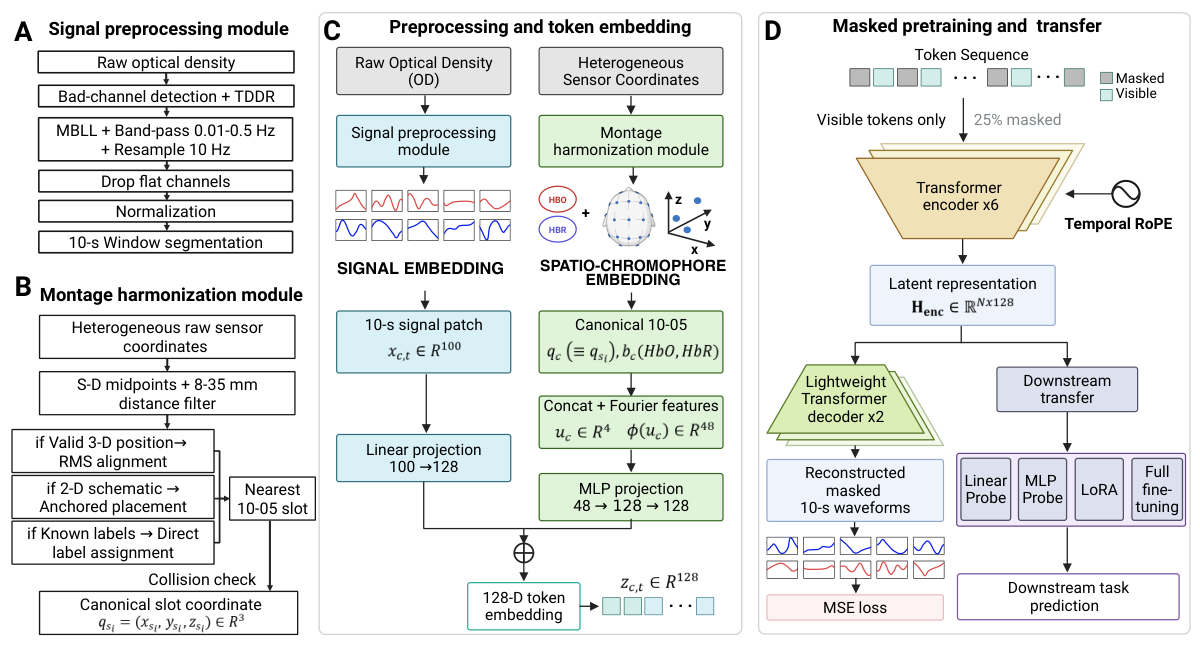
Fig. 2 of Chae et al. (2026), arXiv:2610.36159 (CC BY 4.0). This class is the encoder of panels (C)-(D) with a linear head.#
MtReNIRS (Montage-aligned transferable Representations for fNIRS) is the fNIRS foundation model of Chae et al. [1]: “a montage-aware masked autoencoder, pretrained on 12 public fNIRS datasets spanning 268 subjects and 567 recording hours”. It “jointly encodes the slow hemodynamic nature of fNIRS, chromophore identity and cortical location by mapping heterogeneous montages onto a shared anatomical reference”. A token is one 10-s window of one chromophore channel, tagged with the canonical 10-05 position [2] of its source-detector (S-D) pair and with its chromophore; six Transformer blocks mix all tokens, with the window index as their only time code.
Architectural Overview
With
W = n_times // window_sampleswindows,C = n_chansHbO/HbR rows andD = embed_dim:Windowing:
(batch, C, n_times)is cut into non-overlapping 10-s windows \(x_{c,t}\),(batch, W, C, window_samples); a short last window is cropped (on_non_divisible).Token embedding: each window becomes a token \(z_{c,t}\), the sum of its signal embedding and of the spatio-chromophore embedding of its channel,
(batch, W * C, D).Transformer encoder:
depthpre-norm blocks attend over all channels and windows jointly, then a final LayerNorm; invalid tokens are never attended and are zeroed,(batch, W, C, D).Readout and head:
poolreduces the tokens to(batch, feature_dim)andfinal_layergives(batch, n_outputs).
Macro Components
Token embedding (
embed,_TokenEmbedding).Operations. Signal embedding
embed.signal.proj,nn.Linear(100, 128): “Each 10-s signal segment \(x_{c,t} \in \mathbb{R}^{100}\) was projected by a linear layer to a 128-dimensional signal embedding”. Spatio-chromophore embeddingembed.spatial.mlp,nn.Linear(48, 128), GELU,nn.Linear(128, 128), on six bands of Fourier features [3] of \(u_c = [q_c^\top, b_c]^\top \in \mathbb{R}^4\), the canonical coordinate \(q_c\) of the S-D pair and the chromophore \(b_c\) (0 HbO, 1 HbR):\[\phi(u_c) = \left[\sin(2^k \pi u_{c,j}),\, \cos(2^k \pi u_{c,j}) \right]_{j = 1, \dots, 4}^{k = 0, \dots, 5} \in \mathbb{R}^{48}, \qquad z_{c,t} = W_x x_{c,t} + b_x + \mathrm{MLP}(\phi(u_c)).\]Role. “This embedding lets the encoder distinguish region-specific activity while modeling coupled, often opposing HbO/HbR dynamics.” There is no CLS token and no per-channel table.
Canonical coordinates (
default_coordinates, or thecoordinatesargument offorward()).Operations. \(\hat{q}_c = (q_c - \mu) / \sigma\) with \(\mu\) =
coordinate_centerand \(\sigma\) =coordinate_scale: “We normalized all available canonical coordinates with one center and RMS scale computed from the pretraining corpus.”Role. Before the model, the paper maps every montage to the 10-05 system (Sec. III-B, Eq. 1) and uses “the fixed coordinate \(q_{s_i}\) of assigned slot \(s_i\)”. That alignment and slot assignment (the authors’
mtrenirs.alignment.align) stay outside this class, which reads \(q_c\) fromloc[:3]ofchs_info.
Transformer encoder (
encoder.blocks,encoder.norm;_TransformerBlock,_RotarySelfAttention).Operations. “The encoder contained six pre-layer-normalized Transformer blocks with a 128-dimensional state, four attention heads, a 512-dimensional MLP, and 0.1 dropout. Per-head layer normalization stabilized queries and keys.” With \(y\) the normalized input, a block computes
\[h = z + \mathrm{Drop}\big(\mathrm{Attn}(\mathrm{LN}_1(z))\big), \qquad z' = h + \mathrm{MLP}(\mathrm{LN}_2(h)),\]\[\mathrm{Attn}_n = \sum_m \mathrm{softmax}_m\!\left( \frac{(\mathcal{R}_{t_n} \mathrm{LN}_q(W_q y_n))^\top \mathcal{R}_{t_m} \mathrm{LN}_k(W_k y_m)}{\sqrt{d_h}} + M_m \right) W_v y_m,\]where \(\mathcal{R}_t\) is the rotary rotation [4] of the window index \(t\) with frequencies \(\beta^{-2j/d_h}\), \(\beta\) =
rope_base, and \(M_m = 0\) for a valid key and \(-\infty\) otherwise.Role. “To preserve cross-window order without conflating time with spatial identity, rotary position encoding (RoPE) with base 500 encoded the temporal-window index. All S-D pairs from the same window shared that index; spatial identity entered only through the canonical coordinate embedding.”
Readout and head (
pool,final_layer).Operations.
"temporal_mean"(default): mean over the valid windows, oneembed_dimvector per channel, concatenated;"channel_temporal_mean": mean over the valid windows and channels;"flatten": all tokens. Thennn.Linear.Role. The paper’s linear probe on frozen features (Sec. III-D): “we temporally averaged encoder outputs before classification so that the feature dimensionality remained fixed.”
Temporal, Spatial, and Spectral Encoding
Temporal: within a window, the 100 input weights of the signal projection (no convolution); across windows, RoPE of the window index only. The weights expect 10 Hz and 10-s windows.
Spatial: every row of
xis one chromophore channel, in any order and number; the HbO and HbR rows of one S-D pair share \(q_c\). Rows without a location (NaN or all-zeroloc) are left out of the attention and the pooling.Chromophore: read from MNE’s
coil_typeor the" hbo"/" hbr"name suffix; any other channel (e.g. HbT) raises.
Additional Mechanisms
Masked pretraining (Fig. 2D, Sec. III-C; not part of this class): “we randomly masked 25% of valid tokens and passed only visible tokens to the encoder. A two-block lightweight Transformer decoder reconstructed each masked 10-s waveform”, with a mean squared error over the masked tokens (Eq. 3).
Pretrained Weights
mtrenirs_10s.ptof microsoft/MtReNIRS (commit 16c3082, MIT), the paper’s epoch-95 checkpoint of the 10-s model, is mirrored unchanged at braindecode/mtrenirs-pretrained. It holds the inference encoder only.load_state_dict()takes this payload strictly with the authors’ key names;final_layerkeeps its initialization. It expects 10 Hz HbO/HbR, preprocessed as in Notes, in 100-sample windows, with positions on 10-05 slots:path = hf_hub_download( "braindecode/mtrenirs-pretrained", "mtrenirs_10s.pt", revision="bbc68ce5e00a4515081d900227fc06d111858e75", ) payload = torch.load(path, map_location="cpu", weights_only=True) # raw: MNE Raw with the 10-05 slot positions in loc[:3] model = MtReNIRS(chs_info=raw.info["chs"], n_outputs=3, n_times=100, sfreq=10.0) model.load_state_dict(payload)
Added in version 2.1.
- Parameters:
n_outputs (
int|None) – Number of outputs of the model. This is the number of classes in the case of classification.chs_info (
list[dict] |None) – Information about each individual EEG channel. This should be filled withinfo["chs"]. Refer tomne.Infofor more details.n_times (
int|None) – Number of time samples of the input window.input_window_seconds (
float|None) – Length of the input window in seconds.sfreq (
float|None) – Sampling frequency of the EEG recordings.window_samples (
int) – Samples per token window \(x_{c,t}\); the paper’s “10-s (100-sample) windows” at 10 Hz.embed_dim (
int) – Token and Transformer width, the paper’s “128-dimensional state”.depth (
int) – Number of Transformer blocks.num_heads (
int) – Attention heads;embed_dim // num_headsmust be even for RoPE.mlp_dim (
int) – Hidden width of each block’s feed-forward network.n_fourier_bands (
int) – Fourier bands \(2^k \pi\) per coordinate of \(u_c\) (“six bands of Fourier features”, 48 features).spatial_hidden_dim (
int) – Hidden width of the spatio-chromophore MLP (48 -> 128 -> 128).rope_base (
float) – RoPE base \(\beta\) of the window index.qk_norm (
bool) – Per-head LayerNorm of queries and keys.pool (
Literal['temporal_mean','channel_temporal_mean','flatten']) – Readout of the(batch, n_windows, n_chans, embed_dim)tokens: mean over the valid windows (the paper’s temporal averaging); mean over the valid windows and channels (takesch_mask); or all tokens flattened.on_non_divisible (
Literal['crop','pad','error']) – A short last window is dropped (the reference’sremainder="drop"), zero-padded or refused.coordinate_center (
tuple[float,float,float]) – Centre \(\mu\) (m) subtracted from \(q_c\); the checkpoint’sdata.pos_center.coordinate_scale (
float) – RMS scale \(\sigma\) (m) dividing the centred \(q_c\); the checkpoint’sdata.pos_scale.drop_prob (
float) – Dropout of attention weights, attention output and MLP.activation (
type[Module]) – Activation of the spatio-chromophore MLP and the feed-forward blocks.
- Raises:
ValueError – If some input signal-related parameters are not specified: and can not be inferred.
Notes
Preprocessing (Sec. III-B, Fig. 2A): optical density, temporal derivative distribution repair, modified Beer-Lambert law; “We then band-pass filtered each run from 0.01 to 0.5 Hz, resampled to 10 Hz, and removed flat or abnormally low-variance chromophore channels”; z-score of each chromophore channel over its run, clipped to \([-6, 6]\); downstream windows “[onset, onset + 10 s) without a hemodynamic-response shift”.
Band-pass: the paper gives the band, 0.01 to 0.5 Hz. The released
from_mne_rawuses MNE’s default FIR for it; the replication below used a zero-phase third-order Butterworth,raw.filter(0.01, 0.5, method="iir", iir_params=dict(order=3, ftype="butter")), and reproduces the paper’s numbers (#1564). With MNE’s default FIR, 43.8 % of the window power stays above 0.5 Hz, against 1.1 % with that Butterworth.Differences from the reference implementation: the input is a
(batch, n_chans, n_times)tensor with the montage inchs_info;final_layerandpool="channel_temporal_mean"are added (the reference returns features only); a window with a NaN sample is left out of the attention and of the average; the reference’sremainder="overlap"is not offered. On the released checkpoint, the encoder features equal the authors’MtReNIRSEncoder(MtReNIRS@16c3082) with max-abs difference 0.0.Replication on SujinBak 2019 [5] (30 subjects, left- hand, right-hand and foot tapping) with this port and
mtrenirs_10s.pt(macro-F1, %), under the paper’s protocol: leave-one-subject-out with a linear probe (LP), MLP probe, LoRA, full fine-tuning (Full-FT) and random initialization (Scratch-FT), and within-subject few-shot linear probes.LP
MLP
LoRA
Full-FT
Scratch-FT
2-shot
4-shot
6-shot
8-shot
Paper
67.9
67.2
70.3
70.2
66.7
40.4
46.2
50.0
53.0
Paper SD
17.7
18.6
18.6
19.1
16.2
8.1
11.9
14.2
15.1
Port
68.3
67.4
69.3
69.6
67.8
40.3
46.6
50.4
53.0
References
Hugging Face Hub integration
When the optional
huggingface_hubpackage is installed, all models automatically gain the ability to be pushed to and loaded from the Hugging Face Hub. Install with:pip install braindecode[hub]
Pushing a model to the Hub:
from braindecode.models import MtReNIRS

# Train your model
model = MtReNIRS(n_chans=22, n_outputs=4, n_times=1000)
# ... training code ...

# Push to the Hub; ``datasets`` and ``base_model`` go to the card
model.push_to_hub(
    repo_id="username/my-mtrenirs-model",
    commit_message="Initial model upload",
    model_card_kwargs={"datasets": ["BNCI2014_001"]},
)
Loading a model from the Hub:
from braindecode.models import MtReNIRS

# Load pretrained model
model = MtReNIRS.from_pretrained("username/my-mtrenirs-model")
# Data the weights were trained on, from the Hub model card
print(model.card_data.datasets if model.card_data else None)

# Load with a different number of outputs (head is rebuilt automatically)
model = MtReNIRS.from_pretrained("username/my-mtrenirs-model", n_outputs=4)
Extracting features and replacing the head:
import torch

x = torch.randn(1, model.n_chans, model.n_times)
# Extract encoder features (consistent dict across all models)
out = model(x, return_features=True)
features = out["features"]

# Replace the classification head
model.reset_head(n_outputs=10)
Saving and restoring full configuration:
import json

config = model.get_config()            # all __init__ params
with open("config.json", "w") as f:
    json.dump(config, f)

model2 = MtReNIRS.from_config(config)    # reconstruct (no weights)
All model parameters (both EEG-specific and model-specific such as dropout rates, activation functions, number of filters) are automatically saved to the Hub and restored when loading.
See Loading and Adapting Pretrained Foundation Models for a complete tutorial.
Methods
- encode_windows(x, coordinates=None, ch_mask=None)[source]#
Tokenize the recording and encode its (channel, window) tokens.
- Parameters:
x (
Tensor) – Hemoglobin concentrations,(batch, n_chans, n_times). A NaN sample masks its window.coordinates (
Optional[Tensor]) – \(u_c\) of the channels ofx,(n_chans, 4)or(batch, n_chans, 4): standardized position and chromophore (0 HbO, 1 HbR). NaN positions mark channels without a location.Noneuses the coordinates built fromchs_info.ch_mask (
Optional[Tensor]) –Truefor real channels,(batch, n_chans).
- Return type:
- Returns:
encoded (torch.Tensor) – Encoded tokens,
(batch, n_windows, n_chans, embed_dim); zero where a token is not valid.valid (torch.Tensor) – Validity of each token,
(batch, n_windows, n_chans).
- forward(x, return_features=False, coordinates=None, ch_mask=None)[source]#
Forward pass.
- Parameters:
x (
Tensor) – Hemoglobin concentrations,(batch, n_chans, n_times).return_features (
bool) – Return the pooled features instead of the logits.coordinates (
Optional[Tensor]) – \(u_c\) of the channels ofx, as inencode_windows().ch_mask (
Optional[Tensor]) –Truefor real channels,(batch, n_chans)(check_ch_mask()). Needspool="channel_temporal_mean"; padded channels are left out of the attention and the pooling.
- Returns:
Logits
(batch, n_outputs), or withreturn_featuresa dict withfeatures(batch, feature_dim)andcls_token(None: the model has no class token).- Return type:
- load_state_dict(state_dict, strict=True, assign=False)[source]#
Also takes the official checkpoint (
{"model": ...}); a missing head keeps its init.