
braindecode.models.FNIRSNet#
- class braindecode.models.FNIRSNet(n_outputs=None, n_chans=None, chs_info=None, n_times=None, input_window_seconds=None, sfreq=None, *, n_dhr_filters=4, n_pw_filters=8, dhr_kernel_length=None, activation=<class 'torch.nn.modules.activation.Sigmoid'>)[source]#
fNIRSNet from Wang et al. (2023).
Convolution
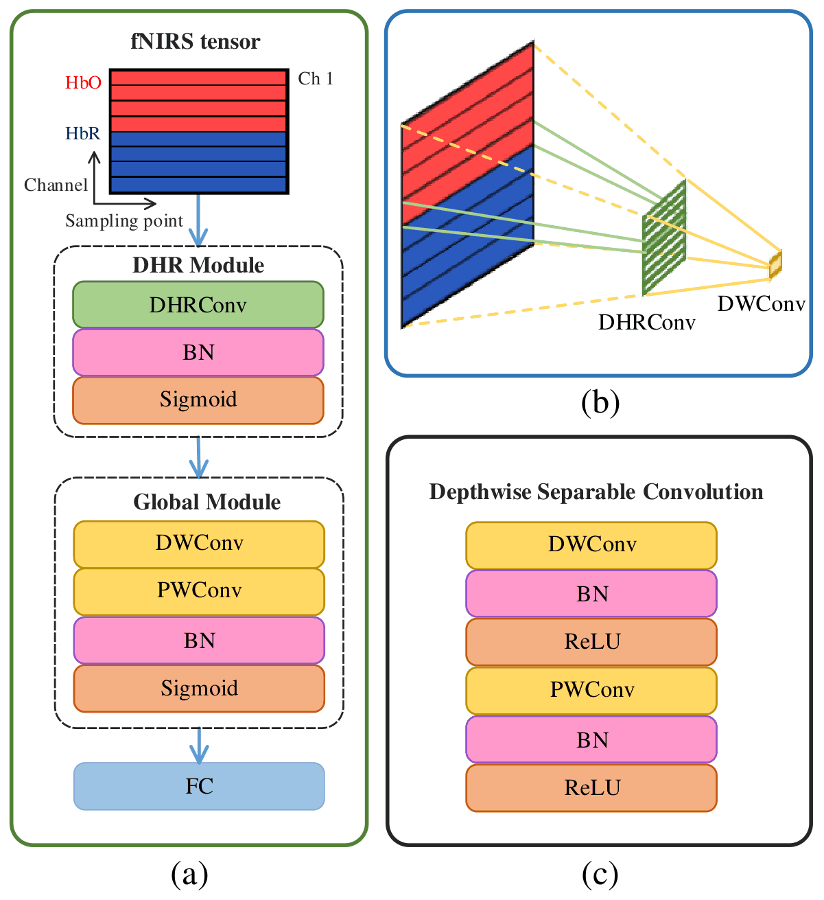
Fig. 2 of Wang et al. (2023), cropped (CC BY 4.0): “(a) Overview architecture of fNIRSNet. (b) Schema of receptive fields. The green and yellow feature maps are the output of DHRConv and DWConv, respectively. […] (c) Depthwise separable convolution.”#
Changes of oxygenated and deoxygenated hemoglobin (HbO, HbR) are “a slow metabolic process manifested as delayed hemodynamic responses”, and the paper [1] argues that deep networks for fNIRS ignore them: “A small kernel with a limited receptive field is challenging to extract the features of delayed hemodynamic responses because there is no significant change in HbO and HbR in small neighborhoods. However, stacking more convolutional layers to obtain larger receptive fields may cause overfitting on limited fNIRS data” (Section I).
fNIRSNet answers with “two core ideas: 1) delayed hemodynamic responses as domain knowledge should be introduced into fNIRS classification models; 2) a simple and efficient model is beneficial to practical applications on limited fNIRS data”. It has “three convolutional layers and one fully connected (FC) layer without pooling, dropout, and other complicated structures”: a convolution whose kernel spans the whole window of one row, then one whose kernel spans all rows. With 4 and 8 filters it has 498 parameters on mental arithmetic (Table III).
Architecture Overview
“fNIRSNet consists of a delayed hemodynamic response module (DHR Module) and a global module” (Section II-B, Table I). With \(C\) =
n_chansrows, \(S\) =n_timessamples, \(F_1\) and \(F_2\) filters, and \(S' = S - k + 1\) (1 for the paper’s kernel width \(k = S\)):input (batch, C, S) to_fnirs_tensor (batch, 1, C, S) DHR Module: conv1 (1 x k), bn1, sigmoid (batch, F_1, C, S') Global Module: conv2.depth_conv (C x 1) (batch, F_1, 1, S') conv2.point_conv (1 x 1), bn2, sigmoid (batch, F_2, 1, S') flatten, final_layer (FC) (batch, n_outputs)
Macro Components
conv1,bn1DHR Module. “Delayed hemodynamic response convolutions (DHRConv) extract the channel-level features of delayed hemodynamic responses.” DHRConv is a standard convolution with \(F_1\) filters of \(1 \times S\): “the width of this kernel equals the number of input sampling points” (Guideline 1). It stays a standard convolution because “the depthwise separable convolution performs poorly in low-dimensional space (the first layer)” (Guideline 2). Batch normalization and a sigmoid follow.conv2,bn2Global Module. A depthwise separable convolution: DWConv, one \(C \times 1\) filter per DHRConv map, “can directly obtain global receptive fields without stacking layers”, and “the \(1 \times 1\) PWConv projects the output of DWConv into a new channel space” with \(F_2\) filters; then batch normalization and a sigmoid. Guideline 2 motivates the factorization by the cost of a standard convolution against a depthwise separable one, for a \(K_h \times K_w\) kernel, \(F_{in}\) input and \(F_{out}\) output channels and an \(M_h \times M_w\) map (Eqs. (2) and (3)):\[K_h K_w F_{in} F_{out} M_h M_w \quad \text{vs.} \quad K_h K_w F_{in} M_h M_w + F_{in} F_{out} M_h M_w ,\]so the global module costs \(F_1 (C + F_2)\) instead of \(F_1 C F_2\), and “increasing the length of input signals only increases the computational cost of DHRConv”.
activationSaturating activations. Guideline 3: “Activation functions with saturated negative values can alleviate information loss in the first layer”; sigmoid, tanh and ELU beat ReLU and leaky ReLU in the ablation of Table VI, and the paper uses the sigmoid.final_layerClassifier. “The feature maps are flattened to 1D vectors and then fed into an FC layer”, without dropout; the paper’s softmax is left to the loss, and the module returns logits.
Temporal, Spatial, and Spectral Encoding
Temporal: one 3 s window of \(S = f \times T\) samples (30 at 10 Hz on MA, 40 at 13.3 Hz on UFFT). DHRConv covers all of it, because the response it targets is long: the paper models it with the canonical hemodynamic response function of three gamma functions (Section II-A, Eq. (1)), whose \(A\), \(\alpha\) and \(\beta\) “control the height and direction, shape, and scale of hemodynamic responses”:
\[h(t) = \sum_{i=1}^{3} A_i \frac{t^{\alpha_i - 1} \beta_i^{\alpha_i} e^{-\beta_i t}}{\Gamma(\alpha_i)} .\]The kernel counts samples, so the model takes no sampling rate.
Spatial: no montage or optode geometry. DWConv mixes all rows at once, since “DHRConv alone cannot aggregate spatial information from multi-channel fNIRS”.
chs_infois not read: the row order must be the one used in training.Chromophores: \(C\) “is twice (two chromophores: HbO and HbR) the number of fNIRS channels” (Section II-B); as in Fig. 2(a) and the authors’ loaders, all HbO rows come first, then all HbR rows.
Spectral: none in the model; the paper band-passes the concentration changes to 0.01-0.1 Hz first (Section III-B).
Pretrained Weights
None: the authors release code, not weights, and the paper trains one model per subject or per left-out subject.
Differences from the reference implementation
xis(batch, n_chans, n_times);to_fnirs_tensoradds the depth axis of the authors’(batch, 1, C, S)input. The modules keep the authors’ names exceptfc, nowfinal_layer;mappingrenamesfc.*, so theirstate_dictloads withstrict=True. Table I lists \(F_2\) filters for DWConv, but the authors’DWSConvand the cost \(F_1 (C + F_2)\) above have \(F_1\) depthwise filters and an \(F_1 \to F_2\) PWConv; this module follows the code, which gives Table III’s parameter counts. Two additions:dhr_kernel_lengthmay be shorter than the window (the authors’ FC layer only fits \(k = S\)), andactivationreplaces the fixed sigmoid. A training batch of one sample runs the BN layers on their running statistics, andch_maskraises aValueError.- Parameters:
n_outputs (
int|None) – Number of outputs of the model. This is the number of classes in the case of classification.chs_info (
list[dict] |None) – Information about each individual EEG channel. This should be filled withinfo["chs"]. Refer tomne.Infofor more details.n_times (
int|None) – Number of time samples of the input window.input_window_seconds (
float|None) – Length of the input window in seconds.sfreq (
float|None) – Sampling frequency of the EEG recordings.n_dhr_filters (
int) – \(F_1\), the DHRConv filters (the authors’num_DHRConv): 4 subject-specific, 16 subject-independent (Section III-D; the authors’LOSO_Train.pyuses 8). “Except for the number of filters \(F_1\) and \(F_2\), fNIRSNet has almost no other hyperparameters.”n_pw_filters (
int) – \(F_2\), the PWConv filters (the authors’num_DWConv): 8 subject-specific, 32 subject-independent (LOSO_Train.py: 16). The paper recommends “setting the value of \(F_2\) to at least twice that of \(F_1\)” (Section IV-F).dhr_kernel_length (
int|None) – DHRConv width \(k\),1 <= k <= n_times;Noneuses \(S\) (Guideline 1). Table IV also tries \(k\) = 10, 20 and 30 on UFFT; the FC layer then reads \(F_2 (S - k + 1)\) values.activation (
type[Module]) – Activation after each BN (the authors’act).
- Raises:
ValueError – If some input signal-related parameters are not specified: and can not be inferred.
Notes
Protocol (Section III, details from the authors’ code): MA [2] (2 classes, 29 subjects, 10 Hz) and UFFT [3] (3 classes, 30 subjects, 13.3 Hz), band-passed 0.01-0.1 Hz, baseline-corrected, cut into 3 s windows with a 1 s step and z-scored. Subject-specific runs use 5-fold CV over trial blocks for 120 epochs, subject-independent runs leave one subject out for 30 epochs; AdamW (lr 0.001), label smoothing 0.1, last-epoch test metrics. Table III gives 498 and 419 parameters for the subject-specific sizes (MA \(C = 72, S = 30\); UFFT \(C = S = 40\)) and 2,370 and 2,051 for the subject-independent ones; this module gives the same counts.
On UFFT, in the authors’ training loops (seeds 0-2), the port and the authors’
fNIRSNetagree within 0.01 point (accuracy / macro-F1 in %; the LOSO runs use the authors’ \(F_1 = 8\), \(F_2 = 16\)):UFFT
Paper, Table II
This port
Authors’ code
Subject-specific
68.67 / 68.02
67.68 / 66.83
67.68 / 66.83
Subject-independent
64.43 / 63.57
64.52 / 63.67
64.51 / 63.67
Added in version 2.1.
References
Hugging Face Hub integration
When the optional
huggingface_hubpackage is installed, all models automatically gain the ability to be pushed to and loaded from the Hugging Face Hub. Install with:pip install braindecode[hub]
Pushing a model to the Hub:
from braindecode.models import FNIRSNet

# Train your model
model = FNIRSNet(n_chans=22, n_outputs=4, n_times=1000)
# ... training code ...

# Push to the Hub; ``datasets`` and ``base_model`` go to the card
model.push_to_hub(
    repo_id="username/my-fnirsnet-model",
    commit_message="Initial model upload",
    model_card_kwargs={"datasets": ["BNCI2014_001"]},
)
Loading a model from the Hub:
from braindecode.models import FNIRSNet

# Load pretrained model
model = FNIRSNet.from_pretrained("username/my-fnirsnet-model")
# Data the weights were trained on, from the Hub model card
print(model.card_data.datasets if model.card_data else None)

# Load with a different number of outputs (head is rebuilt automatically)
model = FNIRSNet.from_pretrained("username/my-fnirsnet-model", n_outputs=4)
Extracting features and replacing the head:
import torch

x = torch.randn(1, model.n_chans, model.n_times)
# Extract encoder features (consistent dict across all models)
out = model(x, return_features=True)
features = out["features"]

# Replace the classification head
model.reset_head(n_outputs=10)
Saving and restoring full configuration:
import json

config = model.get_config()            # all __init__ params
with open("config.json", "w") as f:
    json.dump(config, f)

model2 = FNIRSNet.from_config(config)    # reconstruct (no weights)
All model parameters (both EEG-specific and model-specific such as dropout rates, activation functions, number of filters) are automatically saved to the Hub and restored when loading.
See Loading and Adapting Pretrained Foundation Models for a complete tutorial.
Methods
- forward(x, return_features=False, ch_mask=None)[source]#
Forward pass of the fNIRSNet model.
- Parameters:
- Returns:
Logits with shape
(batch_size, n_outputs), or withreturn_features=Truethe dict{"features", "cls_token"},featuresof shape(batch_size, n_pw_filters * time')andcls_tokenNone.- Return type:
- reset_head(n_outputs)[source]#
Replace the classification head for a new number of outputs.
This is called automatically by
from_pretrained()when the user passes ann_outputsthat differs from the saved config. Override in subclasses that need a model-specific head structure. Implementations keep changed constructor arguments in sync withself._update_init_kwargs, so that a saved model can be loaded back. Implementations requiring positive outputs can also useself._set_n_outputsto validate and record the new value.Examples
>>> from braindecode.models import BENDR
>>> model = BENDR(n_chans=22, n_times=1000, n_outputs=4)
>>> model.reset_head(10)
>>> model.n_outputs
10
Added in version 1.4.