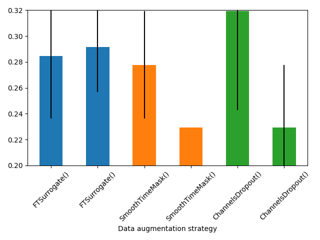
Searching the best data augmentation on BCIC IV 2a Dataset

This tutorial shows how to search data augmentations using braindecode. Indeed, it is known that the best augmentation to use often dependent on the task or phenomenon studied. Here we follow the methodology proposed in [1] on the openly available BCI IV 2a Dataset.

Data Augmentation

Data augmentation could be a step in training deep learning models. For decoding brain signals, recent studies have shown that artificially generating samples may increase the final performance of a deep learning model [1]. Other studies have shown that data augmentation can be used to cast a self-supervised paradigm, presenting a more diverse view of the data, both with pretext tasks and contrastive learning [2].

Data augmentation and self-supervised learning approaches demand an intense comparison to find the best fit with the data. This view is demonstrated in [1] and shows the importance of selecting the right transformation and strength for different type of task considered. Here, we use the augmentation module present in braindecode in the context of trialwise decoding with the BCI IV 2a dataset.

# Authors: Bruno Aristimunha <a.bruno@ufabc.edu.br>
#          Cédric Rommel <cedric.rommel@inria.fr>
# License: BSD (3-clause)

Loading and preprocessing the dataset

Loading

First, we load the data. In this tutorial, we use the functionality of braindecode to load BCI IV competition dataset 1. The dataset is available on the BNCI website. There is 9 subjects recorded with 22 electrodes while doing a motor imagery task, with 144 trials per class. We will load this dataset through the MOABB library.

from skorch.callbacks import LRScheduler

from braindecode import EEGClassifier
from braindecode.datasets import MOABBDataset

subject_id = 3
dataset = MOABBDataset(dataset_name="BNCI2014001", subject_ids=[subject_id])

BNCI2014001 has been renamed to BNCI2014_001. BNCI2014001 will be removed in version 1.1.
The dataset class name 'BNCI2014001' must be an abbreviation of its code 'BNCI2014-001'. See moabb.datasets.base.is_abbrev for more information.

Preprocessing

We apply a bandpass filter, from 4 to 38 Hz to focus motor imagery-related brain activity

from braindecode.preprocessing import (
    exponential_moving_standardize, preprocess, Preprocessor)
from numpy import multiply

low_cut_hz = 4.  # low cut frequency for filtering
high_cut_hz = 38.  # high cut frequency for filtering
# Parameters for exponential moving standardization
factor_new = 1e-3
init_block_size = 1000
# Factor to convert from V to uV
factor = 1e6

In time series targets setup, targets variables are stored in mne.Raw object as channels of type misc. Thus those channels have to be selected for further processing. However, many mne functions ignore misc channels and perform operations only on data channels (see https://mne.tools/stable/glossary.html#term-data-channels).

preprocessors = [
    Preprocessor('pick_types', eeg=True, meg=False, stim=False),  # Keep EEG sensors
    Preprocessor(lambda data: multiply(data, factor)),  # Convert from V to uV
    Preprocessor('filter', l_freq=low_cut_hz, h_freq=high_cut_hz),  # Bandpass filter
    Preprocessor(exponential_moving_standardize,  # Exponential moving standardization
                 factor_new=factor_new, init_block_size=init_block_size)
]

preprocess(dataset, preprocessors, n_jobs=-1)

/home/runner/work/braindecode/braindecode/braindecode/preprocessing/preprocess.py:55: UserWarning: Preprocessing choices with lambda functions cannot be saved.
  warn('Preprocessing choices with lambda functions cannot be saved.')

<braindecode.datasets.moabb.MOABBDataset object at 0x7f45416e9210>

Extracting windows

Now we cut out compute windows, the inputs for the deep networks during training. We use the braindecode function for this, provinding parameters to define how trials should be used.

from braindecode.preprocessing import create_windows_from_events
from skorch.helper import SliceDataset
from numpy import array

trial_start_offset_seconds = -0.5
# Extract sampling frequency, check that they are same in all datasets
sfreq = dataset.datasets[0].raw.info['sfreq']
assert all([ds.raw.info['sfreq'] == sfreq for ds in dataset.datasets])
# Calculate the trial start offset in samples.
trial_start_offset_samples = int(trial_start_offset_seconds * sfreq)

windows_dataset = create_windows_from_events(
    dataset,
    trial_start_offset_samples=trial_start_offset_samples,
    trial_stop_offset_samples=0,
    preload=True,
)

Split dataset into train and valid

Following the split defined in the BCI competition

splitted = windows_dataset.split('session')
train_set = splitted['0train']  # Session train
eval_set = splitted['1test']  # Session evaluation

Defining a list of transforms

In this tutorial, we will use three categories of augmentations. This categorization has been proposed by [1] to explain and aggregate the several possibilities of augmentations in EEG, being them:

1. Frequency domain augmentations,

2. Time domain augmentations,

3. Spatial domain augmentations.

From this same paper, we selected the best augmentations in each type: FTSurrogate, SmoothTimeMask, ChannelsDropout, respectively.

For each augmentation, we adjustable two values from a range for one parameter inside the transformation.

It is important to remember that you can increase the range. For that, we need to define three lists of transformations and range for the parameter ∆φmax in FTSurrogate where ∆φmax ∈ [0, 2π); for ∆t in SmoothTimeMask is ∆t ∈ [0, 2]; For the method ChannelsDropout, we analyse the parameter p_drop ∈ [0, 1].

from numpy import linspace
from braindecode.augmentation import FTSurrogate, SmoothTimeMask, ChannelsDropout

seed = 20200220

transforms_freq = [FTSurrogate(probability=0.5, phase_noise_magnitude=phase_freq,
                               random_state=seed) for phase_freq in linspace(0, 1, 2)]

transforms_time = [SmoothTimeMask(probability=0.5, mask_len_samples=int(sfreq * second),
                                  random_state=seed) for second in linspace(0.1, 2, 2)]

transforms_spatial = [ChannelsDropout(probability=0.5, p_drop=prob,
                                      random_state=seed) for prob in linspace(0, 1, 2)]

Training a model with data augmentation

Now that we know how to instantiate three list of Transforms, it is time to learn how to use them to train a model and try to search the best for the dataset. Let’s first create a model for search a parameter.

Create model

The model to be trained is defined as usual.

import torch

from braindecode.util import set_random_seeds
from braindecode.models import ShallowFBCSPNet

cuda = torch.cuda.is_available()  # check if GPU is available, if True chooses to use it
device = 'cuda' if cuda else 'cpu'
if cuda:
    torch.backends.cudnn.benchmark = True

Set random seed to be able to roughly reproduce results Note that with cudnn benchmark set to True, GPU indeterminism may still make results substantially different between runs. To obtain more consistent results at the cost of increased computation time, you can set cudnn_benchmark=False in set_random_seeds or remove torch.backends.cudnn.benchmark = True

seed = 20200220
set_random_seeds(seed=seed, cuda=cuda)

n_classes = 4
classes = list(range(n_classes))
# Extract number of chans and time steps from dataset
n_channels = train_set[0][0].shape[0]
input_window_samples = train_set[0][0].shape[1]

model = ShallowFBCSPNet(
    n_channels,
    n_classes,
    input_window_samples=input_window_samples,
    final_conv_length='auto',
)

/home/runner/work/braindecode/braindecode/braindecode/models/base.py:23: UserWarning: ShallowFBCSPNet: 'input_window_samples' is depreciated. Use 'n_times' instead.
  warnings.warn(
/home/runner/work/braindecode/braindecode/braindecode/models/base.py:180: UserWarning: LogSoftmax final layer will be removed! Please adjust your loss function accordingly (e.g. CrossEntropyLoss)!
  warnings.warn("LogSoftmax final layer will be removed! " +

Create an EEGClassifier with the desired augmentation

In order to train with data augmentation, a custom data loader can be for the training. Multiple transforms can be passed to it and will be applied sequentially to the batched data within the AugmentedDataLoader object.

from braindecode.augmentation import AugmentedDataLoader

# Send model to GPU
if cuda:
    model.cuda()

The model is now trained as in the trial-wise example. The AugmentedDataLoader is used as the train iterator and the list of transforms are passed as arguments.

lr = 0.0625 * 0.01
weight_decay = 0

batch_size = 64
n_epochs = 2

clf = EEGClassifier(
    model,
    iterator_train=AugmentedDataLoader,  # This tells EEGClassifier to use a custom DataLoader
    iterator_train__transforms=[],  # This sets is handled by GridSearchCV
    criterion=torch.nn.NLLLoss,
    optimizer=torch.optim.AdamW,
    train_split=None,  # GridSearchCV will control the split and train/validation over the dataset
    optimizer__lr=lr,
    optimizer__weight_decay=weight_decay,
    batch_size=batch_size,
    callbacks=[
        'accuracy',
        ('lr_scheduler', LRScheduler('CosineAnnealingLR', T_max=n_epochs - 1)),
    ],
    device=device,
    classes=classes
)

To use the skorch framework, it is necessary to transform the windows dataset using the module SliceData. Also, it is mandatory to eval the generator of the training.

train_X = SliceDataset(train_set, idx=0)
train_y = array(list(SliceDataset(train_set, idx=1)))

Given the trialwise approach, here we use the KFold approach and GridSearchCV.

from sklearn.model_selection import KFold, GridSearchCV

cv = KFold(n_splits=2, shuffle=True, random_state=seed)
fit_params = {'epochs': n_epochs}

transforms = transforms_freq + transforms_time + transforms_spatial

param_grid = {
    'iterator_train__transforms': transforms,
}

clf.verbose = 0

search = GridSearchCV(
    estimator=clf,
    param_grid=param_grid,
    cv=cv,
    return_train_score=True,
    scoring='accuracy',
    refit=True,
    verbose=1,
    error_score='raise')

search.fit(train_X, train_y, **fit_params)

Fitting 2 folds for each of 6 candidates, totalling 12 fits

GridSearchCV(cv=KFold(n_splits=2, random_state=20200220, shuffle=True),
             error_score='raise',
             estimator=<class 'braindecode.classifier.EEGClassifier'>[uninitialized](
  module=============================================================================================================================================
  Layer (type (var_name):depth-idx)        Input Shape               Ou...
  Estimated Total Size (MB): 0.50
  ============================================================================================================================================,
),
             param_grid={'iterator_train__transforms': [FTSurrogate(),
                                                        FTSurrogate(),
                                                        SmoothTimeMask(),
                                                        SmoothTimeMask(),
                                                        ChannelsDropout(),
                                                        ChannelsDropout()]},
             return_train_score=True, scoring='accuracy', verbose=1)

In a Jupyter environment, please rerun this cell to show the HTML representation or trust the notebook.
On GitHub, the HTML representation is unable to render, please try loading this page with nbviewer.org.

Analysing the best fit

Next, just perform an analysis of the best fit, and the parameters, remembering the order that was adjusted.

import pandas as pd
import numpy as np

search_results = pd.DataFrame(search.cv_results_)

best_run = search_results[search_results['rank_test_score'] == 1].squeeze()
best_aug = best_run['params']
validation_score = np.around(best_run['mean_test_score'] * 100, 2).mean()
training_score = np.around(best_run['mean_train_score'] * 100, 2).mean()

report_message = 'Best augmentation is saved in best_aug which gave a mean validation accuracy' + \
                 'of {}% (train accuracy of {}%).'.format(validation_score, training_score)

print(report_message)

eval_X = SliceDataset(eval_set, idx=0)
eval_y = SliceDataset(eval_set, idx=1)
score = search.score(eval_X, eval_y)
print(f'Eval accuracy is {score * 100:.2f}%.')

Best augmentation is saved in best_aug which gave a mean validation accuracyof 27.78% (train accuracy of 28.47%).
Eval accuracy is 25.00%.

Plot results

import matplotlib.pyplot as plt

fig, ax = plt.subplots()
search_results.plot.bar(
    x="param_iterator_train__transforms", y="mean_train_score", yerr="std_train_score",
    rot=45, color=["C0", "C0", "C1", "C1", "C2", "C2"], legend=None, ax=ax)
ax.set_xlabel("Data augmentation strategy")
ax.set_ylim(0.2, 0.32)
plt.tight_layout()

References

[1] (1,2,3,4)

Rommel, C., Paillard, J., Moreau, T., & Gramfort, A. (2022) Data augmentation for learning predictive models on EEG: a systematic comparison. https://arxiv.org/abs/2206.14483

[2]

Banville, H., Chehab, O., Hyvärinen, A., Engemann, D. A., & Gramfort, A. (2021). Uncovering the structure of clinical EEG signals with self-supervised learning. Journal of Neural Engineering, 18(4), 046020.

Estimated memory usage: 522 MB