Sleep staging on the Sleep Physionet dataset using Chambon2018 network

This tutorial shows how to train and test a sleep staging neural network with Braindecode. We adapt the time distributed approach of [1] to learn on sequences of EEG windows using the openly accessible Sleep Physionet dataset [2] [3].

# Authors: Hubert Banville <hubert.jbanville@gmail.com>
#
# License: BSD (3-clause)

Loading and preprocessing the dataset

Loading

First, we load the data using the braindecode.datasets.sleep_physionet.SleepPhysionet class. We load two recordings from two different individuals: we will use the first one to train our network and the second one to evaluate performance (as in the MNE sleep staging example).

from numbers import Integral
from braindecode.datasets import SleepPhysionet

subject_ids = [0, 1]
dataset = SleepPhysionet(
    subject_ids=subject_ids, recording_ids=[2], crop_wake_mins=30)

Preprocessing

Next, we preprocess the raw data. We convert the data to microvolts and apply a lowpass filter. We omit the downsampling step of [1] as the Sleep Physionet data is already sampled at a lower 100 Hz.

from braindecode.preprocessing import preprocess, Preprocessor
from numpy import multiply

high_cut_hz = 30
factor = 1e6

preprocessors = [
    Preprocessor(lambda data: multiply(data, factor), apply_on_array=True),  # Convert from V to uV
    Preprocessor('filter', l_freq=None, h_freq=high_cut_hz)
]

# Transform the data
preprocess(dataset, preprocessors)

/home/runner/work/braindecode/braindecode/braindecode/preprocessing/preprocess.py:55: UserWarning: Preprocessing choices with lambda functions cannot be saved.
  warn('Preprocessing choices with lambda functions cannot be saved.')

<braindecode.datasets.sleep_physionet.SleepPhysionet object at 0x7f4541467fd0>

Extract windows

We extract 30-s windows to be used in the classification task.

from braindecode.preprocessing import create_windows_from_events

mapping = {  # We merge stages 3 and 4 following AASM standards.
    'Sleep stage W': 0,
    'Sleep stage 1': 1,
    'Sleep stage 2': 2,
    'Sleep stage 3': 3,
    'Sleep stage 4': 3,
    'Sleep stage R': 4
}

window_size_s = 30
sfreq = 100
window_size_samples = window_size_s * sfreq

windows_dataset = create_windows_from_events(
    dataset,
    trial_start_offset_samples=0,
    trial_stop_offset_samples=0,
    window_size_samples=window_size_samples,
    window_stride_samples=window_size_samples,
    preload=True,
    mapping=mapping
)

Window preprocessing

We also preprocess the windows by applying channel-wise z-score normalization in each window.

from sklearn.preprocessing import scale as standard_scale

preprocess(windows_dataset, [Preprocessor(standard_scale, channel_wise=True)])

<braindecode.datasets.base.BaseConcatDataset object at 0x7f4542374550>

Split dataset into train and valid

We split the dataset into training and validation set taking every other subject as train or valid.

split_ids = dict(train=subject_ids[::2], valid=subject_ids[1::2])
splits = windows_dataset.split(split_ids)
train_set, valid_set = splits["train"], splits["valid"]

Create sequence samplers

Following the time distributed approach of [1], we need to provide our neural network with sequences of windows, such that the embeddings of multiple consecutive windows can be concatenated and provided to a final classifier. We can achieve this by defining Sampler objects that return sequences of window indices. To simplify the example, we train the whole model end-to-end on sequences, rather than using the two-step approach of [1] (i.e. training the feature extractor on single windows, then freezing its weights and training the classifier).

import numpy as np
from braindecode.samplers import SequenceSampler

n_windows = 3  # Sequences of 3 consecutive windows
n_windows_stride = 3  # Maximally overlapping sequences

train_sampler = SequenceSampler(
    train_set.get_metadata(), n_windows, n_windows_stride, randomize=True
)
valid_sampler = SequenceSampler(valid_set.get_metadata(), n_windows, n_windows_stride)

# Print number of examples per class
print('Training examples: ', len(train_sampler))
print('Validation examples: ', len(valid_sampler))

Training examples:  372
Validation examples:  383

We also implement a transform to extract the label of the center window of a sequence to use it as target.

# Use label of center window in the sequence
def get_center_label(x):
    if isinstance(x, Integral):
        return x
    return x[np.ceil(len(x) / 2).astype(int)] if len(x) > 1 else x


train_set.target_transform = get_center_label
valid_set.target_transform = get_center_label

Finally, since some sleep stages appear a lot more often than others (e.g. most of the night is spent in the N2 stage), the classes are imbalanced. To avoid overfitting on the more frequent classes, we compute weights that we will provide to the loss function when training.

from sklearn.utils import compute_class_weight

y_train = [train_set[idx][1] for idx in train_sampler]
class_weights = compute_class_weight('balanced', classes=np.unique(y_train), y=y_train)

Create model

We can now create the deep learning model. In this tutorial, we use the sleep staging architecture introduced in [1], which is a four-layer convolutional neural network. We use the time distributed version of the model, where the feature vectors of a sequence of windows are concatenated and passed to a linear layer for classification.

import torch
from torch import nn
from braindecode.util import set_random_seeds
from braindecode.models import SleepStagerChambon2018, TimeDistributed

cuda = torch.cuda.is_available()  # check if GPU is available
device = 'cuda' if torch.cuda.is_available() else 'cpu'
if cuda:
    torch.backends.cudnn.benchmark = True
# Set random seed to be able to roughly reproduce results
# Note that with cudnn benchmark set to True, GPU indeterminism
# may still make results substantially different between runs.
# To obtain more consistent results at the cost of increased computation time,
# you can set `cudnn_benchmark=False` in `set_random_seeds`
# or remove `torch.backends.cudnn.benchmark = True`
set_random_seeds(seed=31, cuda=cuda)

n_classes = 5
# Extract number of channels and time steps from dataset
n_channels, input_size_samples = train_set[0][0].shape

feat_extractor = SleepStagerChambon2018(
    n_channels,
    sfreq,
    n_outputs=n_classes,
    n_times=input_size_samples,
    return_feats=True
)

model = nn.Sequential(
    TimeDistributed(feat_extractor),  # apply model on each 30-s window
    nn.Sequential(  # apply linear layer on concatenated feature vectors
        nn.Flatten(start_dim=1),
        nn.Dropout(0.5),
        nn.Linear(feat_extractor.len_last_layer * n_windows, n_classes)
    )
)

# Send model to GPU
if cuda:
    model.cuda()

Training

We can now train our network. braindecode.EEGClassifier is a braindecode object that is responsible for managing the training of neural networks. It inherits from skorch.NeuralNetClassifier, so the training logic is the same as in Skorch.

Note

We use different hyperparameters from [1], as these hyperparameters were optimized on a different dataset (MASS SS3) and with a different number of recordings. Generally speaking, it is recommended to perform hyperparameter optimization if reusing this code on a different dataset or with more recordings.

from skorch.helper import predefined_split
from skorch.callbacks import EpochScoring
from braindecode import EEGClassifier

lr = 1e-3
batch_size = 32
n_epochs = 10

train_bal_acc = EpochScoring(
    scoring='balanced_accuracy', on_train=True, name='train_bal_acc',
    lower_is_better=False)
valid_bal_acc = EpochScoring(
    scoring='balanced_accuracy', on_train=False, name='valid_bal_acc',
    lower_is_better=False)
callbacks = [
    ('train_bal_acc', train_bal_acc),
    ('valid_bal_acc', valid_bal_acc)
]

clf = EEGClassifier(
    model,
    criterion=torch.nn.CrossEntropyLoss,
    criterion__weight=torch.Tensor(class_weights).to(device),
    optimizer=torch.optim.Adam,
    iterator_train__shuffle=False,
    iterator_train__sampler=train_sampler,
    iterator_valid__sampler=valid_sampler,
    train_split=predefined_split(valid_set),  # using valid_set for validation
    optimizer__lr=lr,
    batch_size=batch_size,
    callbacks=callbacks,
    device=device,
    classes=np.unique(y_train),
)
# Model training for a specified number of epochs. `y` is None as it is already
# supplied in the dataset.
clf.fit(train_set, y=None, epochs=n_epochs)

  epoch    train_bal_acc    train_loss    valid_acc    valid_bal_acc    valid_loss     dur
-------  ---------------  ------------  -----------  ---------------  ------------  ------
      1           0.2136        1.5768       0.0888           0.2000        1.6372  1.5977
      2           0.2036        1.4788       0.0888           0.2000        1.6676  1.4921
      3           0.2324        1.4033       0.0966           0.2102        1.6337  1.5023
      4           0.2888        1.3407       0.1149           0.2465        1.6790  1.5318
      5           0.3993        1.2126       0.4517           0.4013        1.6235  1.6800
      6           0.5294        1.0967       0.2768           0.4076        1.6179  1.5747
      7           0.5755        0.9662       0.5927           0.5671        1.3689  1.5097
      8           0.6251        0.8904       0.7076           0.5786        1.2952  1.4943
      9           0.6877        0.8148       0.7154           0.5876        1.3450  1.5740
     10           0.6860        0.7449       0.5196           0.5269        1.6322  1.5012

<class 'braindecode.classifier.EEGClassifier'>[initialized](
  module_=Sequential(
    (0): TimeDistributed(
      (module): SleepStagerChambon2018(
        (spatial_conv): Conv2d(1, 2, kernel_size=(2, 1), stride=(1, 1))
        (feature_extractor): Sequential(
          (0): Conv2d(1, 8, kernel_size=(1, 50), stride=(1, 1), padding=(0, 25))
          (1): Identity()
          (2): ReLU()
          (3): MaxPool2d(kernel_size=(1, 13), stride=(1, 13), padding=0, dilation=1, ceil_mode=False)
          (4): Conv2d(8, 8, kernel_size=(1, 50), stride=(1, 1), padding=(0, 25))
          (5): Identity()
          (6): ReLU()
          (7): MaxPool2d(kernel_size=(1, 13), stride=(1, 13), padding=0, dilation=1, ceil_mode=False)
        )
      )
    )
    (1): Sequential(
      (0): Flatten(start_dim=1, end_dim=-1)
      (1): Dropout(p=0.5, inplace=False)
      (2): Linear(in_features=816, out_features=5, bias=True)
    )
  ),
)

Plot results

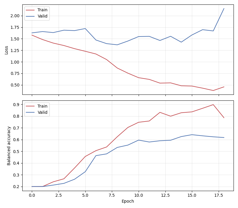
We use the history stored by Skorch during training to plot the performance of the model throughout training. Specifically, we plot the loss and the balanced balanced accuracy for the training and validation sets.

import matplotlib.pyplot as plt
import pandas as pd

# Extract loss and balanced accuracy values for plotting from history object
df = pd.DataFrame(clf.history.to_list())
df.index.name = "Epoch"
fig, (ax1, ax2) = plt.subplots(2, 1, figsize=(8, 7), sharex=True)
df[['train_loss', 'valid_loss']].plot(color=['r', 'b'], ax=ax1)
df[['train_bal_acc', 'valid_bal_acc']].plot(color=['r', 'b'], ax=ax2)
ax1.set_ylabel('Loss')
ax2.set_ylabel('Balanced accuracy')
ax1.legend(['Train', 'Valid'])
ax2.legend(['Train', 'Valid'])
fig.tight_layout()
plt.show()

Finally, we also display the confusion matrix and classification report:

from sklearn.metrics import confusion_matrix, classification_report
from braindecode.visualization import plot_confusion_matrix

y_true = [valid_set[[i]][1][0] for i in range(len(valid_sampler))]
y_pred = clf.predict(valid_set)

confusion_mat = confusion_matrix(y_true, y_pred)

plot_confusion_matrix(confusion_mat=confusion_mat,
                      class_names=['Wake', 'N1', 'N2', 'N3', 'REM'])

print(classification_report(y_true, y_pred))

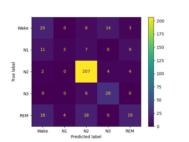
              precision    recall  f1-score   support

           0       0.14      0.33      0.20        61
           1       0.19      0.14      0.16        21
           2       0.56      0.34      0.42       194
           3       0.26      0.27      0.26        75
           4       0.03      0.03      0.03        32

    accuracy                           0.28       383
   macro avg       0.24      0.22      0.21       383
weighted avg       0.37      0.28      0.31       383

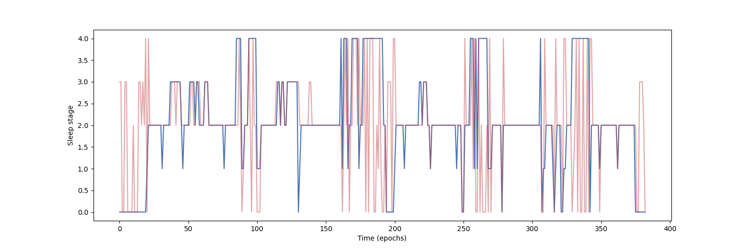
Finally, we can also visualize the hypnogram of the recording we used for validation, with the predicted sleep stages overlaid on top of the true sleep stages. We can see that the model cannot correctly identify the different sleep stages with this amount of training.

import matplotlib.pyplot as plt

fig, ax = plt.subplots(figsize=(15, 5))
ax.plot(y_true, color='b', label='Expert annotations')
ax.plot(y_pred.flatten(), color='r', label='Predict annotations', alpha=0.5)
ax.set_xlabel('Time (epochs)')
ax.set_ylabel('Sleep stage')

Text(150.22222222222223, 0.5, 'Sleep stage')

Our model was able to learn despite the low amount of data that was available (only two recordings in this example) and reached a balanced accuracy of about 36% in a 5-class classification task (chance-level = 20%) on held-out data.

Note

To further improve performance, more recordings should be included in the training set, and hyperparameters should be selected accordingly. Increasing the sequence length was also shown in [1] to help improve performance, especially when few EEG channels are available.

References

[1] (1,2,3,4,5,6,7)

Chambon, S., Galtier, M., Arnal, P., Wainrib, G. and Gramfort, A. (2018)A Deep Learning Architecture for Temporal Sleep Stage Classification Using Multivariate and Multimodal Time Series. IEEE Trans. on Neural Systems and Rehabilitation Engineering 26: (758-769)

[2]

B Kemp, AH Zwinderman, B Tuk, HAC Kamphuisen, JJL Oberyé. Analysis of a sleep-dependent neuronal feedback loop: the slow-wave microcontinuity of the EEG. IEEE-BME 47(9):1185-1194 (2000).

[3]

Goldberger AL, Amaral LAN, Glass L, Hausdorff JM, Ivanov PCh, Mark RG, Mietus JE, Moody GB, Peng C-K, Stanley HE. (2000) PhysioBank, PhysioToolkit, and PhysioNet: Components of a New Research Resource for Complex Physiologic Signals. Circulation 101(23):e215-e220

Estimated memory usage: 10 MB