Self-supervised learning on EEG with relative positioning

This example shows how to train a neural network with self-supervision on sleep EEG data. We follow the relative positioning approach of [1] on the openly accessible Sleep Physionet dataset [2] [3].

Self-supervised learning

Self-supervised learning (SSL) is a learning paradigm that leverages unlabelled data to train neural networks. First, neural networks are trained on a “pretext task” which uses unlabelled data only. The pretext task is designed based on a prior understanding of the data under study (e.g., EEG has an underlying autocorrelation structure) and such that the processing required to perform well on this pretext task is related to the processing required to perform well on another task of interest. Once trained, these neural networks can be reused as feature extractors or weight initialization in a “downstream task”, which is the task that we are actually interested in (e.g., sleep staging). The pretext task step can help reduce the quantity of labelled data needed to perform well on the downstream task and/or improve downstream performance as compared to a strictly supervised approach [1].

Here, we use relative positioning (RP) as our pretext task, and perform sleep staging as our downstream task. RP is a simple SSL task, in which a neural network is trained to predict whether two randomly sampled EEG windows are close or far apart in time. This method was shown to yield physiologically- and clinically-relevant features and to boost classification performance in low-labels data regimes [1].

# Authors: Hubert Banville <hubert.jbanville@gmail.com>
#
# License: BSD (3-clause)


random_state = 87
n_jobs = 1

Loading and preprocessing the dataset

Loading the raw recordings

First, we load a few recordings from the Sleep Physionet dataset. Running this example with more recordings should yield better representations and downstream classification performance.

from braindecode.datasets.sleep_physionet import SleepPhysionet

dataset = SleepPhysionet(
    subject_ids=[0, 1, 2], recording_ids=[1], crop_wake_mins=30)

Preprocessing

Next, we preprocess the raw data. We convert the data to microvolts and apply a lowpass filter. Since the Sleep Physionet data is already sampled at 100 Hz we don’t need to apply resampling.

from braindecode.preprocessing.preprocess import preprocess, Preprocessor
from numpy import multiply

high_cut_hz = 30
# Factor to convert from V to uV
factor = 1e6

preprocessors = [
    Preprocessor(lambda data: multiply(data, factor)),  # Convert from V to uV
    Preprocessor('filter', l_freq=None, h_freq=high_cut_hz, n_jobs=n_jobs)
]

# Transform the data
preprocess(dataset, preprocessors)

/home/runner/work/braindecode/braindecode/braindecode/preprocessing/preprocess.py:55: UserWarning: Preprocessing choices with lambda functions cannot be saved.
  warn('Preprocessing choices with lambda functions cannot be saved.')

<braindecode.datasets.sleep_physionet.SleepPhysionet object at 0x7f454279da80>

Extracting windows

We extract 30-s windows to be used in both the pretext and downstream tasks. As RP (and SSL in general) don’t require labelled data, the pretext task could be performed using unlabelled windows extracted with braindecode.datautil.windower.create_fixed_length_window(). Here however, purely for convenience, we directly extract labelled windows so that we can reuse them in the sleep staging downstream task later.

from braindecode.preprocessing.windowers import create_windows_from_events

window_size_s = 30
sfreq = 100
window_size_samples = window_size_s * sfreq

mapping = {  # We merge stages 3 and 4 following AASM standards.
    'Sleep stage W': 0,
    'Sleep stage 1': 1,
    'Sleep stage 2': 2,
    'Sleep stage 3': 3,
    'Sleep stage 4': 3,
    'Sleep stage R': 4
}

windows_dataset = create_windows_from_events(
    dataset, trial_start_offset_samples=0, trial_stop_offset_samples=0,
    window_size_samples=window_size_samples,
    window_stride_samples=window_size_samples, preload=True, mapping=mapping)

Preprocessing windows

We also preprocess the windows by applying channel-wise z-score normalization.

from sklearn.preprocessing import scale as standard_scale

preprocess(windows_dataset, [Preprocessor(standard_scale, channel_wise=True)])

<braindecode.datasets.base.BaseConcatDataset object at 0x7f4540a2a710>

Splitting dataset into train, valid and test sets

We randomly split the recordings by subject into train, validation and testing sets. We further define a new Dataset class which can receive a pair of indices and return the corresponding windows. This will be needed when training and evaluating on the pretext task.

import numpy as np
from sklearn.model_selection import train_test_split
from braindecode.datasets import BaseConcatDataset

subjects = np.unique(windows_dataset.description['subject'])
subj_train, subj_test = train_test_split(
    subjects, test_size=0.4, random_state=random_state)
subj_valid, subj_test = train_test_split(
    subj_test, test_size=0.5, random_state=random_state)


class RelativePositioningDataset(BaseConcatDataset):
    """BaseConcatDataset with __getitem__ that expects 2 indices and a target.
    """

    def __init__(self, list_of_ds):
        super().__init__(list_of_ds)
        self.return_pair = True

    def __getitem__(self, index):
        if self.return_pair:
            ind1, ind2, y = index
            return (super().__getitem__(ind1)[0],
                    super().__getitem__(ind2)[0]), y
        else:
            return super().__getitem__(index)

    @property
    def return_pair(self):
        return self._return_pair

    @return_pair.setter
    def return_pair(self, value):
        self._return_pair = value


split_ids = {'train': subj_train, 'valid': subj_valid, 'test': subj_test}
splitted = dict()
for name, values in split_ids.items():
    splitted[name] = RelativePositioningDataset(
        [ds for ds in windows_dataset.datasets
         if ds.description['subject'] in values])

Creating samplers

Next, we need to create samplers. These samplers will be used to randomly sample pairs of examples to train and validate our model with self-supervision.

The RP samplers have two main hyperparameters. tau_pos and tau_neg control the size of the “positive” and “negative” contexts, respectively. Pairs of windows that are separated by less than tau_pos samples will be given a label of 1, while pairs of windows that are separated by more than tau_neg samples will be given a label of 0. Here, we use the same values as in [1], i.e., `tau_pos`= 1 min and `tau_neg`= 15 mins.

The samplers also control the number of pairs to be sampled (defined with n_examples). This number can be large to help regularize the pretext task training, for instance 2,000 pairs per recording as in [1]. Here, we use a lower number of 250 pairs per recording to reduce training time.

from braindecode.samplers import RelativePositioningSampler

tau_pos, tau_neg = int(sfreq * 60), int(sfreq * 15 * 60)
n_examples_train = 250 * len(splitted['train'].datasets)
n_examples_valid = 250 * len(splitted['valid'].datasets)
n_examples_test = 250 * len(splitted['test'].datasets)

train_sampler = RelativePositioningSampler(
    splitted['train'].get_metadata(), tau_pos=tau_pos, tau_neg=tau_neg,
    n_examples=n_examples_train, same_rec_neg=True, random_state=random_state)
valid_sampler = RelativePositioningSampler(
    splitted['valid'].get_metadata(), tau_pos=tau_pos, tau_neg=tau_neg,
    n_examples=n_examples_valid, same_rec_neg=True,
    random_state=random_state).presample()
test_sampler = RelativePositioningSampler(
    splitted['test'].get_metadata(), tau_pos=tau_pos, tau_neg=tau_neg,
    n_examples=n_examples_test, same_rec_neg=True,
    random_state=random_state).presample()

Creating the model

We can now create the deep learning model. In this tutorial, we use a modified version of the sleep staging architecture introduced in [4] - a four-layer convolutional neural network - as our embedder. We change the dimensionality of the last layer to obtain a 100-dimension embedding, use 16 convolutional channels instead of 8, and add batch normalization after both temporal convolution layers.

We further wrap the model into a siamese architecture using the # ContrastiveNet class defined below. This allows us to train the feature extractor end-to-end.

import torch
from torch import nn
from braindecode.util import set_random_seeds
from braindecode.models import SleepStagerChambon2018

device = 'cuda' if torch.cuda.is_available() else 'cpu'
if device == 'cuda':
    torch.backends.cudnn.benchmark = True
# Set random seed to be able to roughly reproduce results
# Note that with cudnn benchmark set to True, GPU indeterminism
# may still make results substantially different between runs.
# To obtain more consistent results at the cost of increased computation time,
# you can set `cudnn_benchmark=False` in `set_random_seeds`
# or remove `torch.backends.cudnn.benchmark = True`
set_random_seeds(seed=random_state, cuda=device == 'cuda')

# Extract number of channels and time steps from dataset
n_channels, input_size_samples = windows_dataset[0][0].shape
emb_size = 100
classes = list(range(5))

emb = SleepStagerChambon2018(
    n_channels,
    sfreq,
    n_outputs=emb_size,
    n_conv_chs=16,
    n_times=input_size_samples,
    dropout=0,
    apply_batch_norm=True,
)


class ContrastiveNet(nn.Module):
    """Contrastive module with linear layer on top of siamese embedder.

    Parameters
    ----------
    emb : nn.Module
        Embedder architecture.
    emb_size : int
        Output size of the embedder.
    dropout : float
        Dropout rate applied to the linear layer of the contrastive module.
    """

    def __init__(self, emb, emb_size, dropout=0.5):
        super().__init__()
        self.emb = emb
        self.clf = nn.Sequential(
            nn.Dropout(dropout),
            nn.Linear(emb_size, 1)
        )

    def forward(self, x):
        x1, x2 = x
        z1, z2 = self.emb(x1), self.emb(x2)
        return self.clf(torch.abs(z1 - z2)).flatten()


model = ContrastiveNet(emb, emb_size).to(device)

Training

We can now train our network on the pretext task. We use similar hyperparameters as in [1], but reduce the number of epochs and increase the learning rate to account for the smaller setting of this example.

import os

from skorch.helper import predefined_split
from skorch.callbacks import Checkpoint, EarlyStopping, EpochScoring
from braindecode import EEGClassifier

lr = 5e-3
batch_size = 128  # 512 if data large enough
n_epochs = 25
num_workers = 0 if n_jobs <= 1 else n_jobs

cp = Checkpoint(dirname='', f_criterion=None, f_optimizer=None, f_history=None)
early_stopping = EarlyStopping(patience=10)
train_acc = EpochScoring(
    scoring='accuracy', on_train=True, name='train_acc', lower_is_better=False)

callbacks = [
    ('cp', cp),
    ('patience', early_stopping),
    ('train_acc', train_acc),
]

clf = EEGClassifier(
    model,
    criterion=torch.nn.BCEWithLogitsLoss,
    optimizer=torch.optim.Adam,
    max_epochs=n_epochs,
    iterator_train__shuffle=False,
    iterator_train__sampler=train_sampler,
    iterator_valid__sampler=valid_sampler,
    iterator_train__num_workers=num_workers,
    iterator_valid__num_workers=num_workers,
    train_split=predefined_split(splitted['valid']),
    optimizer__lr=lr,
    batch_size=batch_size,
    callbacks=callbacks,
    device=device,
    classes=classes,
)
# Model training for a specified number of epochs. `y` is None as it is already
# supplied in the dataset.
clf.fit(splitted['train'], y=None)
clf.load_params(checkpoint=cp)  # Load the model with the lowest valid_loss

os.remove('./params.pt')  # Delete parameters file

  epoch    train_acc    train_loss    valid_acc    valid_loss    cp     dur
-------  -----------  ------------  -----------  ------------  ----  ------
      1       0.5234        0.7013       0.6680        0.6320     +  1.1152
      2       0.5938        0.7149       0.4880        0.8358        0.9011
      3       0.4922        1.0040       0.6440        0.6172     +  0.9228
      4       0.5234        0.7031       0.6120        0.5990     +  0.9178
      5       0.5391        0.6751       0.5920        0.6213        0.8892
      6       0.6719        0.6227       0.5920        0.6263        0.8797
      7       0.6562        0.6309       0.6240        0.6117        0.8809
      8       0.6641        0.6272       0.6480        0.5950     +  0.8784
      9       0.6328        0.6238       0.6680        0.5797     +  0.8630
     10       0.6406        0.6177       0.6800        0.5746     +  0.8675
     11       0.6250        0.6323       0.7040        0.5787        0.8569
     12       0.6094        0.6281       0.6760        0.5772        0.8705
     13       0.6328        0.6422       0.6880        0.5790        0.8659
     14       0.6406        0.5920       0.6840        0.5765        0.8664
     15       0.6562        0.6170       0.6920        0.5730     +  0.8699
     16       0.7578        0.5608       0.6960        0.5676     +  0.8702
     17       0.6875        0.5936       0.7120        0.5612     +  0.8605
     18       0.7734        0.5472       0.7080        0.5500     +  0.8628
     19       0.7656        0.5245       0.7120        0.5400     +  0.8698
     20       0.6641        0.5641       0.7160        0.5333     +  0.9171
     21       0.7422        0.5307       0.7200        0.5272     +  0.8718
     22       0.7109        0.5499       0.7360        0.5211     +  0.8695
     23       0.6250        0.6259       0.7400        0.5164     +  0.8774
     24       0.7031        0.5712       0.7400        0.5120     +  0.8637
     25       0.7109        0.5030       0.7280        0.5120        0.8741

Visualizing the results

Inspecting pretext task performance

We plot the loss and pretext task performance for the training and validation sets.

import matplotlib.pyplot as plt
import pandas as pd

# Extract loss and balanced accuracy values for plotting from history object
df = pd.DataFrame(clf.history.to_list())

df['train_acc'] *= 100
df['valid_acc'] *= 100

ys1 = ['train_loss', 'valid_loss']
ys2 = ['train_acc', 'valid_acc']
styles = ['-', ':']
markers = ['.', '.']

fig, ax1 = plt.subplots(figsize=(8, 3))
ax2 = ax1.twinx()
for y1, y2, style, marker in zip(ys1, ys2, styles, markers):
    ax1.plot(df['epoch'], df[y1], ls=style, marker=marker, ms=7,
             c='tab:blue', label=y1)
    ax2.plot(df['epoch'], df[y2], ls=style, marker=marker, ms=7,
             c='tab:orange', label=y2)

ax1.tick_params(axis='y', labelcolor='tab:blue')
ax1.set_ylabel('Loss', color='tab:blue')
ax2.tick_params(axis='y', labelcolor='tab:orange')
ax2.set_ylabel('Accuracy [%]', color='tab:orange')
ax1.set_xlabel('Epoch')

lines1, labels1 = ax1.get_legend_handles_labels()
lines2, labels2 = ax2.get_legend_handles_labels()
ax2.legend(lines1 + lines2, labels1 + labels2)

plt.tight_layout()

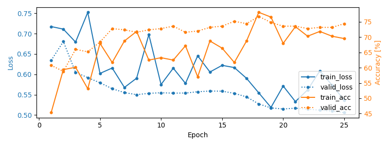
We also display the confusion matrix and classification report for the pretext task:

from sklearn.metrics import confusion_matrix
from sklearn.metrics import classification_report

# Switch to the test sampler
clf.iterator_valid__sampler = test_sampler
y_pred = clf.forward(splitted['test'], training=False) > 0
y_true = [y for _, _, y in test_sampler]

print(confusion_matrix(y_true, y_pred))
print(classification_report(y_true, y_pred))

[[90 31]
 [41 88]]
              precision    recall  f1-score   support

         0.0       0.69      0.74      0.71       121
         1.0       0.74      0.68      0.71       129

    accuracy                           0.71       250
   macro avg       0.71      0.71      0.71       250
weighted avg       0.71      0.71      0.71       250

Using the learned representation for sleep staging

We can now use the trained convolutional neural network as a feature extractor. We perform sleep stage classification from the learned feature representation using a linear logistic regression classifier.

from torch.utils.data import DataLoader
from sklearn.metrics import balanced_accuracy_score
from sklearn.linear_model import LogisticRegression
from sklearn.preprocessing import StandardScaler
from sklearn.pipeline import make_pipeline

# Extract features with the trained embedder
data = dict()
for name, split in splitted.items():
    split.return_pair = False  # Return single windows
    loader = DataLoader(split, batch_size=batch_size, num_workers=num_workers)
    with torch.no_grad():
        feats = [emb(batch_x.to(device)).cpu().numpy()
                 for batch_x, _, _ in loader]
    data[name] = (np.concatenate(feats), split.get_metadata()['target'].values)

# Initialize the logistic regression model
log_reg = LogisticRegression(
    penalty='l2', C=1.0, class_weight='balanced', solver='lbfgs',
    multi_class='multinomial', random_state=random_state)
clf_pipe = make_pipeline(StandardScaler(), log_reg)

# Fit and score the logistic regression
clf_pipe.fit(*data['train'])
train_y_pred = clf_pipe.predict(data['train'][0])
valid_y_pred = clf_pipe.predict(data['valid'][0])
test_y_pred = clf_pipe.predict(data['test'][0])

train_bal_acc = balanced_accuracy_score(data['train'][1], train_y_pred)
valid_bal_acc = balanced_accuracy_score(data['valid'][1], valid_y_pred)
test_bal_acc = balanced_accuracy_score(data['test'][1], test_y_pred)

print('Sleep staging performance with logistic regression:')
print(f'Train bal acc: {train_bal_acc:0.4f}')
print(f'Valid bal acc: {valid_bal_acc:0.4f}')
print(f'Test bal acc: {test_bal_acc:0.4f}')

print('Results on test set:')
print(confusion_matrix(data['test'][1], test_y_pred))
print(classification_report(data['test'][1], test_y_pred))

/home/runner/.local/lib/python3.10/site-packages/sklearn/linear_model/_logistic.py:460: ConvergenceWarning: lbfgs failed to converge (status=1):
STOP: TOTAL NO. of ITERATIONS REACHED LIMIT.

Increase the number of iterations (max_iter) or scale the data as shown in:
    https://scikit-learn.org/stable/modules/preprocessing.html
Please also refer to the documentation for alternative solver options:
    https://scikit-learn.org/stable/modules/linear_model.html#logistic-regression
  n_iter_i = _check_optimize_result(
Sleep staging performance with logistic regression:
Train bal acc: 0.8924
Valid bal acc: 0.5215
Test bal acc: 0.6011
Results on test set:
[[107  26   3   4   2]
 [  7  75   9   2  16]
 [ 70  60 350   2  80]
 [  0   0  55  50   0]
 [  0  77  14   0  79]]
              precision    recall  f1-score   support

           0       0.58      0.75      0.66       142
           1       0.32      0.69      0.43       109
           2       0.81      0.62      0.70       562
           3       0.86      0.48      0.61       105
           4       0.45      0.46      0.46       170

    accuracy                           0.61      1088
   macro avg       0.60      0.60      0.57      1088
weighted avg       0.68      0.61      0.62      1088

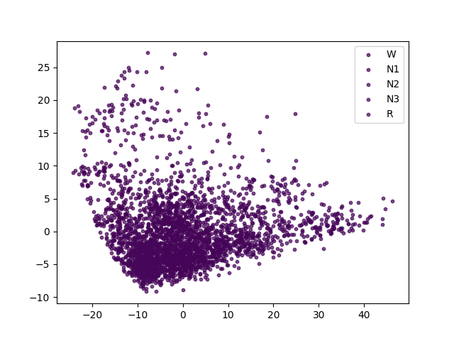
The balanced accuracy is much higher than chance-level (i.e., 20% for our 5-class classification problem). Finally, we perform a quick 2D visualization of the feature space using a PCA:

from sklearn.decomposition import PCA
from matplotlib import cm

X = np.concatenate([v[0] for k, v in data.items()])
y = np.concatenate([v[1] for k, v in data.items()])

pca = PCA(n_components=2)
# tsne = TSNE(n_components=2)
components = pca.fit_transform(X)

fig, ax = plt.subplots()
colors = cm.get_cmap('viridis', 5)(range(5))
for i, stage in enumerate(['W', 'N1', 'N2', 'N3', 'R']):
    mask = y == i
    ax.scatter(components[mask, 0], components[mask, 1], s=10, alpha=0.7,
               color=colors[i], label=stage)
ax.legend()

/home/runner/work/braindecode/braindecode/examples/advanced_training/plot_relative_positioning.py:472: MatplotlibDeprecationWarning: The get_cmap function was deprecated in Matplotlib 3.7 and will be removed two minor releases later. Use ``matplotlib.colormaps[name]`` or ``matplotlib.colormaps.get_cmap(obj)`` instead.
  colors = cm.get_cmap('viridis', 5)(range(5))

<matplotlib.legend.Legend object at 0x7f45409fac20>

We see that there is sleep stage-related structure in the embedding. A nonlinear projection method (e.g., tSNE, UMAP) might yield more insightful visualizations. Using a similar approach, the embedding space could also be explored with respect to subject-level features, e.g., age and sex.

Conclusion

In this example, we used self-supervised learning (SSL) as a way to learn representations from unlabelled raw EEG data. Specifically, we used the relative positioning (RP) pretext task to train a feature extractor on a subset of the Sleep Physionet dataset. We then reused these features in a downstream sleep staging task. We achieved reasonable downstream performance and further showed with a 2D projection that the learned embedding space contained sleep-related structure.

Many avenues could be taken to improve on these results. For instance, using the entire Sleep Physionet dataset or training on larger datasets should help the feature extractor learn better representations during the pretext task. Other SSL tasks such as those described in [1] could further help discover more powerful features.

References

[1] (1,2,3,4,5,6,7)

Banville, H., Chehab, O., Hyvärinen, A., Engemann, D. A., & Gramfort, A. (2020). Uncovering the structure of clinical EEG signals with self-supervised learning. arXiv preprint arXiv:2007.16104.

[2]

Kemp, B., Zwinderman, A. H., Tuk, B., Kamphuisen, H. A., & Oberye, J. J. (2000). Analysis of a sleep-dependent neuronal feedback loop: the slow-wave microcontinuity of the EEG. IEEE Transactions on Biomedical Engineering, 47(9), 1185-1194.

[3]

Goldberger, A. L., Amaral, L. A., Glass, L., Hausdorff, J. M., Ivanov, P. C., Mark, R. G., … & Stanley, H. E. (2000). PhysioBank, PhysioToolkit, and PhysioNet: components of a new research resource for complex physiologic signals. circulation, 101(23), e215-e220.

[4]

Chambon, S., Galtier, M., Arnal, P., Wainrib, G. and Gramfort, A. (2018)A Deep Learning Architecture for Temporal Sleep Stage Classification Using Multivariate and Multimodal Time Series. IEEE Trans. on Neural Systems and Rehabilitation Engineering 26: (758-769)

Estimated memory usage: 199 MB