Note
Go to the end to download the full example code
Fingers flexion decoding on BCIC IV 4 ECoG Dataset#
This tutorial shows you how to train and test deep learning models with Braindecode on ECoG BCI IV competition dataset 4. For this dataset we will predict 5 regression targets corresponding to flexion of each finger. The targets were recorded as a time series (each 25 Hz), so this tutorial is an example of time series target prediction.
# Authors: Maciej Sliwowski <maciek.sliwowski@gmail.com>
#          Mohammed Fattouh <mo.fattouh@gmail.com>
#
# License: BSD (3-clause)
Loading and preparing the dataset#
Loading#
First, we load the data. In this tutorial, we use the functionality of braindecode to load BCI IV competition dataset 4. The dataset is available as a part of ECoG library: https://searchworks.stanford.edu/view/zk881ps0522
The dataset contains ECoG signal and time series of 5 targets corresponding to each finger flexion. This is different than standard decoding setup for EEG with multiple trials and usually one target per trial. Here, fingers flexions change in time and are recorded with sampling frequency equals to 25 Hz.
If this dataset is used please cite [1].
[1] Miller, Kai J. “A library of human electrocorticographic data and analyses. “Nature human behaviour 3, no. 11 (2019): 1225-1235. https://doi.org/10.1038/s41562-019-0678-3
import numpy as np

from braindecode.datasets import BCICompetitionIVDataset4

subject_id = 1
dataset = BCICompetitionIVDataset4(subject_ids=[subject_id])
Preprocessing#
Now we apply preprocessing like bandpass filtering to our dataset. You can either apply functions provided by mne.Raw or mne.Epochs or apply your own functions, either to the MNE object or the underlying numpy array.
Note
Preprocessing steps are taken from a standard EEG processing pipeline. The only change is the cutoff frequency of the filter. For a proper ECoG decoding other preprocessing steps may be needed.
Note
These prepocessings are now directly applied to the loaded data, and not on-the-fly applied as transformations in PyTorch-libraries like torchvision.
from braindecode.preprocessing import (Preprocessor,
                                       exponential_moving_standardize,
                                       preprocess)

low_cut_hz = 1.  # low cut frequency for filtering
high_cut_hz = 200.  # high cut frequency for filtering, for ECoG higher than for EEG
# Parameters for exponential moving standardization
factor_new = 1e-3
init_block_size = 1000
We select only first 30 seconds from each dataset to limit time and memory to run this example. To obtain results on the whole datasets you should remove this line.
preprocess(dataset, [Preprocessor('crop', tmin=0, tmax=30)])
<braindecode.datasets.bcicomp.BCICompetitionIVDataset4 object at 0x7f45411a7af0>
In time series targets setup, targets variables are stored in mne.Raw object as channels of type misc. Thus those channels have to be selected for further processing. However, many mne functions ignore misc channels and perform operations only on data channels (see https://mne.tools/stable/glossary.html#term-data-channels).
preprocessors = [
    Preprocessor('pick_types', ecog=True, misc=True),
    Preprocessor(lambda x: x / 1e6, picks='ecog'),  # Convert from V to uV
    Preprocessor('filter', l_freq=low_cut_hz, h_freq=high_cut_hz),  # Bandpass filter
    Preprocessor(exponential_moving_standardize,  # Exponential moving standardization
                 factor_new=factor_new, init_block_size=init_block_size, picks='ecog')
]

# Transform the data
preprocess(dataset, preprocessors)

# Extract sampling frequency, check that they are same in all datasets
sfreq = dataset.datasets[0].raw.info['sfreq']
assert all([ds.raw.info['sfreq'] == sfreq for ds in dataset.datasets])
# Extract target sampling frequency
target_sfreq = dataset.datasets[0].raw.info['temp']['target_sfreq']
/home/runner/work/braindecode/braindecode/braindecode/preprocessing/preprocess.py:55: UserWarning: Preprocessing choices with lambda functions cannot be saved.
  warn('Preprocessing choices with lambda functions cannot be saved.')
Cut Compute Windows#
Now we cut out compute windows, the inputs for the deep networks during training. In the case of trialwise decoding of time series targets, we just have to decide about length windows that will be selected from the signal preceding each target. We use different windowing function than in standard trialwise decoding as our targets are stored as target channels in mne.Raw.
from braindecode.preprocessing import create_windows_from_target_channels

windows_dataset = create_windows_from_target_channels(
    dataset,
    window_size_samples=1000,
    preload=False,
    last_target_only=True
)
We select only the thumb’s finger flexion to create one model per finger.
Note
Methods to predict all 5 fingers flexion with the same model may be cnosidered as well. We encourage you to find your own way to use braindecode models to predict finers fexions.
windows_dataset.target_transform = lambda x: x[0: 1]
Split dataset into train, valid, and test#
We can easily split the dataset using additional info stored in the
description attribute, in this case session column. We select train dataset
for training and validation and test for final evaluation.
We can split train dataset into training and validation datasets using
sklearn.model_selection.train_test_split and torch.utils.data.Subset.
import torch
from sklearn.model_selection import train_test_split

idx_train, idx_valid = train_test_split(np.arange(len(train_set)),
                                        random_state=100,
                                        test_size=0.2,
                                        shuffle=False)

valid_set = torch.utils.data.Subset(train_set, idx_valid)
train_set = torch.utils.data.Subset(train_set, idx_train)
Create model#
Now we create the deep learning model! Braindecode comes with some predefined convolutional neural network architectures for raw time-domain EEG. Here, we use the shallow ConvNet model from Deep learning with convolutional neural networks for EEG decoding and visualization. These models are pure PyTorch deep learning models, therefore to use your own model, it just has to be a normal PyTorch nn.Module.
from braindecode.models import ShallowFBCSPNet
from braindecode.util import set_random_seeds

cuda = torch.cuda.is_available()  # check if GPU is available, if True chooses to use it
device = 'cuda' if cuda else 'cpu'
if cuda:
    torch.backends.cudnn.benchmark = True
# Set random seed to be able to roughly reproduce results
# Note that with cudnn benchmark set to True, GPU indeterminism
# may still make results substantially different between runs.
# To obtain more consistent results at the cost of increased computation time,
# you can set `cudnn_benchmark=False` in `set_random_seeds`
# or remove `torch.backends.cudnn.benchmark = True`
seed = 20200220
set_random_seeds(seed=seed, cuda=cuda)

n_out_chans = train_set[0][1].shape[0]
# Extract number of chans and time steps from dataset
n_chans = train_set[0][0].shape[0]
input_window_samples = 1000  # 1 second long windows

model = ShallowFBCSPNet(
    n_chans,
    n_out_chans,
    input_window_samples=input_window_samples,
    final_conv_length='auto',
    add_log_softmax=False,
)

# Send model to GPU
if cuda:
    model.cuda()
/home/runner/work/braindecode/braindecode/braindecode/models/base.py:23: UserWarning: ShallowFBCSPNet: 'input_window_samples' is depreciated. Use 'n_times' instead.
  warnings.warn(
Training#
Now we train the network! EEGRegressor is a Braindecode object responsible for managing the training of neural networks. It inherits from skorch.NeuralNetRegressor, so the training logic is the same as in Skorch.
Note
In this tutorial, we use some default parameters that we have found to work well for EEG motor decoding, however we strongly encourage you to perform your own hyperparameter and preprocessing optimization using cross validation on your training data.
from skorch.callbacks import EpochScoring, LRScheduler
from skorch.helper import predefined_split
from mne import set_log_level

from braindecode import EEGRegressor

# These values we found good for shallow network for EEG MI decoding:
lr = 0.0625 * 0.01
weight_decay = 0
batch_size = 64
n_epochs = 2


# Function to compute Pearson correlation coefficient
def pearson_r_score(net, dataset, y):
    preds = net.predict(dataset)
    corr_coeffs = []
    for i in range(y.shape[1]):
        corr_coeffs.append(np.corrcoef(y[:, i], preds[:, i])[0, 1])
    return np.mean(corr_coeffs)


regressor = EEGRegressor(
    model,
    criterion=torch.nn.MSELoss,
    optimizer=torch.optim.AdamW,
    train_split=predefined_split(valid_set),  # using valid_set for validation,
    optimizer__lr=lr,
    optimizer__weight_decay=weight_decay,
    batch_size=batch_size,
    callbacks=[
        'r2',
        ('valid_pearson_r', EpochScoring(pearson_r_score, lower_is_better=False, on_train=False,
                                         name='valid_pearson_r')),
        ('train_pearson_r', EpochScoring(pearson_r_score, lower_is_better=False, on_train=True,
                                         name='train_pearson_r')),
        ("lr_scheduler", LRScheduler('CosineAnnealingLR', T_max=n_epochs - 1)),
    ],
    device=device,
)
set_log_level(verbose='WARNING')
Model training for a specified number of epochs. y is None as it is already supplied
in the dataset.
regressor.fit(train_set, y=None, epochs=n_epochs)
  epoch    train_loss    train_pearson_r    train_r2    valid_loss    valid_pearson_r    valid_r2      lr     dur
-------  ------------  -----------------  ----------  ------------  -----------------  ----------  ------  ------
      1        2.5083             0.1251     -0.5570        5.7337            -0.1507     -1.6139  0.0006  6.3995
      2        1.7986             0.3712     -0.3153        5.2582            -0.1510     -1.3971  0.0000  6.2028
Obtaining predictions and targets for the test, train, and validation dataset
preds_test = regressor.predict(test_set)
y_test = np.stack([data[1] for data in test_set])
preds_train = regressor.predict(train_set)
y_train = np.stack([data[1] for data in train_set])
preds_valid = regressor.predict(valid_set)
y_valid = np.stack([data[1] for data in valid_set])
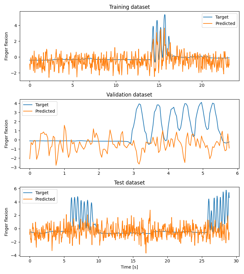
Plot Results#
We plot target and predicted finger flexion on training, validation, and test sets.
Note
The model is trained and validated on limited dataset (to decrease the time needed to run this example) which does not contain diverse dataset in terms of fingers flexions and may cause overfitting. To obtain better results use whole dataset as well as improve the decoding pipeline which may be not optimal for ECoG.
import matplotlib.pyplot as plt
import pandas as pd
from matplotlib.lines import Line2D

fig, axes = plt.subplots(3, 1, figsize=(8, 9))

axes[0].set_title('Training dataset')
axes[0].plot(np.arange(0, y_train.shape[0]) / target_sfreq, y_train[:, 0], label='Target')
axes[0].plot(np.arange(0, preds_train.shape[0]) / target_sfreq, preds_train[:, 0],
             label='Predicted')
axes[0].set_ylabel('Finger flexion')
axes[0].legend()

axes[1].set_title('Validation dataset')
axes[1].plot(np.arange(0, y_valid.shape[0]) / target_sfreq, y_valid[:, 0], label='Target')
axes[1].plot(np.arange(0, preds_valid.shape[0]) / target_sfreq, preds_valid[:, 0],
             label='Predicted')
axes[1].set_ylabel('Finger flexion')
axes[1].legend()

axes[2].set_title('Test dataset')
axes[2].plot(np.arange(0, y_test.shape[0]) / target_sfreq, y_test[:, 0], label='Target')
axes[2].plot(np.arange(0, preds_test.shape[0]) / target_sfreq, preds_test[:, 0], label='Predicted')
axes[2].set_xlabel('Time [s]')
axes[2].set_ylabel('Finger flexion')
axes[2].legend()
plt.tight_layout()
We can compute correlation coefficients for each finger
corr_coeffs = []
for dim in range(y_test.shape[1]):
    corr_coeffs.append(
        np.corrcoef(preds_test[:, dim], y_test[:, dim])[0, 1]
    )
print('Correlation coefficient for each dimension: ', np.round(corr_coeffs, 2))
Correlation coefficient for each dimension: [0.1]
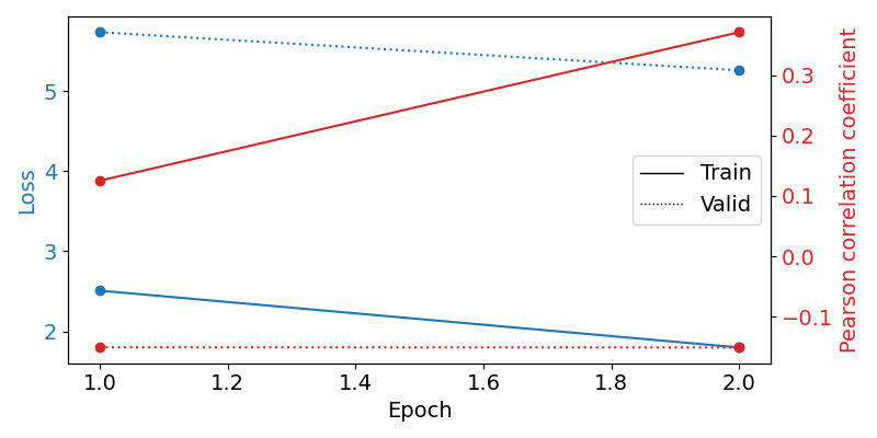
Now we use the history stored by Skorch throughout training to plot accuracy and loss curves. Extract loss and accuracy values for plotting from history object
results_columns = ['train_loss', 'valid_loss', 'train_pearson_r', 'valid_pearson_r']
df = pd.DataFrame(regressor.history[:, results_columns], columns=results_columns,
                  index=regressor.history[:, 'epoch'])

fig, ax1 = plt.subplots(figsize=(8, 4))
df.loc[:, ['train_loss', 'valid_loss']].plot(
    ax=ax1, style=['-', ':'], marker='o', color='tab:blue', legend=False, fontsize=14)

ax1.tick_params(axis='y', labelcolor='tab:blue', labelsize=14)
ax1.set_ylabel("Loss", color='tab:blue', fontsize=14)

ax2 = ax1.twinx()  # instantiate a second axes that shares the same x-axis

df.loc[:, ['train_pearson_r', 'valid_pearson_r']].plot(
    ax=ax2, style=['-', ':'], marker='o', color='tab:red', legend=False)
ax2.tick_params(axis='y', labelcolor='tab:red', labelsize=14)
ax2.set_ylabel("Pearson correlation coefficient", color='tab:red', fontsize=14)
ax1.set_xlabel("Epoch", fontsize=14)

# where some data has already been plotted to ax
handles = []
handles.append(Line2D([0], [0], color='black', linewidth=1, linestyle='-',
                      label='Train'))
handles.append(Line2D([0], [0], color='black', linewidth=1, linestyle=':',
                      label='Valid'))
plt.legend(handles, [h.get_label() for h in handles], fontsize=14, loc='center right')
plt.tight_layout()
Total running time of the script: (0 minutes 25.104 seconds)
Estimated memory usage: 214 MB