How to train, test and tune your model?

This tutorial shows you how to properly train, tune and test your deep learning models with Braindecode. We will use the BCIC IV 2a dataset [1] as a showcase example.

The methods shown can be applied to any standard supervised trial-based decoding setting. This tutorial will include additional parts of code like loading and preprocessing of data, defining a model, and other details which are not exclusive to this page (see Cropped Decoding Tutorial). Therefore we will not further elaborate on these parts and you can feel free to skip them.

In general, we distinguish between “usual” training and evaluation and hyperparameter search. The tutorial is therefore split into two parts, one for the three different training schemes and one for the two different hyperparameter tuning methods.

Why should I care about model evaluation?

Short answer: To produce reliable results!

In machine learning, we usually follow the scheme of splitting the data into two parts, training and testing sets. It sounds like a simple division, right? But the story does not end here.

• What are model’s parameters?

Model’s parameters are learnable weights which are used in the extraction of the relevant features and in performing the final inference. In the context of deep learning, these are usually fully connected weights, convolutional kernels, biases, etc.

• What are model’s hyperparameters?

Model’s hyperparameters are used to set the capacity (size) of the model and to guide the parameter learning process. In the context of deep learning, examples of the hyperparameters are the number of convolutional layers and the number of convolutional kernels in each of them, the number and size of the fully connected weights, choice of the optimizer and its learning rate, the number of training epochs, choice of the nonlinearities, etc.

While developing a ML model you usually have to adjust and tune hyperparameters of your model or pipeline (e.g., number of layers, learning rate, number of epochs). Deep learning models usually have many free parameters; they could be considered as complex models with many degrees of freedom. If you kept using the test dataset to evaluate your adjustment, you would run into data leakage.

This means that if you use the test set to adjust the hyperparameters of your model, the model implicitly learns or memorizes the test set. Therefore, the trained model is no longer independent of the test set (even though it was never used for training explicitly!). If you perform any hyperparameter tuning, you need a third split, the so-called validation set.

This tutorial shows the three basic schemes for training and evaluating the model as well as two methods to tune your hyperparameters.

Warning

You might recognize that the accuracy gets better throughout the experiments of this tutorial. The reason behind that is that we always use the same model with the same parameters in every segment to keep the tutorial short and readable. If you do your own experiments you always have to reinitialize the model before training.

Loading and preprocessing of data, defining a model, etc.

Loading data

In this example, we load the BCI Competition IV 2a data [1], for one subject (subject id 3), using braindecode’s wrapper to load via MOABB library [2].

from braindecode.datasets import MOABBDataset

subject_id = 3
dataset = MOABBDataset(dataset_name="BNCI2014001", subject_ids=[subject_id])

BNCI2014001 has been renamed to BNCI2014_001. BNCI2014001 will be removed in version 1.1.
The dataset class name 'BNCI2014001' must be an abbreviation of its code 'BNCI2014-001'. See moabb.datasets.base.is_abbrev for more information.

Preprocessing data

In this example, preprocessing includes signal rescaling, the bandpass filtering (low and high cut-off frequencies are 4 and 38 Hz) and the standardization using the exponential moving mean and variance.

import numpy as np

from braindecode.preprocessing import (
    exponential_moving_standardize,
    preprocess,
    Preprocessor,
)

low_cut_hz = 4.0  # low cut frequency for filtering
high_cut_hz = 38.0  # high cut frequency for filtering
# Parameters for exponential moving standardization
factor_new = 1e-3
init_block_size = 1000

preprocessors = [
    Preprocessor("pick_types", eeg=True, meg=False, stim=False),  # Keep EEG sensors
    Preprocessor(
        lambda data, factor: np.multiply(data, factor),  # Convert from V to uV
        factor=1e6,
    ),
    Preprocessor("filter", l_freq=low_cut_hz, h_freq=high_cut_hz),  # Bandpass filter
    Preprocessor(
        exponential_moving_standardize,  # Exponential moving standardization
        factor_new=factor_new,
        init_block_size=init_block_size,
    ),
]

# Preprocess the data
preprocess(dataset, preprocessors, n_jobs=-1)

/home/runner/work/braindecode/braindecode/braindecode/preprocessing/preprocess.py:55: UserWarning: Preprocessing choices with lambda functions cannot be saved.
  warn('Preprocessing choices with lambda functions cannot be saved.')

<braindecode.datasets.moabb.MOABBDataset object at 0x7f45456962c0>

Extraction of the Windows

Extraction of the trials (windows) from the time series is based on the events inside the dataset. One event is the demarcation of the stimulus or the beginning of the trial. In this example, we want to analyse 0.5 [s] long before the corresponding event and the duration of the event itself. #Therefore, we set the trial_start_offset_seconds to -0.5 [s] and the trial_stop_offset_seconds to 0 [s].

We extract from the dataset the sampling frequency, which is the same for all datasets in this case, and we tested it.

Note

The trial_start_offset_seconds and trial_stop_offset_seconds are defined in seconds and need to be converted into samples (multiplication with the sampling frequency), relative to the event. This variable is dataset dependent.

from braindecode.preprocessing import create_windows_from_events

trial_start_offset_seconds = -0.5
# Extract sampling frequency, check that they are same in all datasets
sfreq = dataset.datasets[0].raw.info["sfreq"]
assert all([ds.raw.info["sfreq"] == sfreq for ds in dataset.datasets])
# Calculate the window start offset in samples.
trial_start_offset_samples = int(trial_start_offset_seconds * sfreq)

# Create windows using braindecode function for this. It needs parameters to
# define how windows should be used.
windows_dataset = create_windows_from_events(
    dataset,
    trial_start_offset_samples=trial_start_offset_samples,
    trial_stop_offset_samples=0,
    preload=True,
)

Used Annotations descriptions: ['feet', 'left_hand', 'right_hand', 'tongue']
Used Annotations descriptions: ['feet', 'left_hand', 'right_hand', 'tongue']
Used Annotations descriptions: ['feet', 'left_hand', 'right_hand', 'tongue']
Used Annotations descriptions: ['feet', 'left_hand', 'right_hand', 'tongue']
Used Annotations descriptions: ['feet', 'left_hand', 'right_hand', 'tongue']
Used Annotations descriptions: ['feet', 'left_hand', 'right_hand', 'tongue']
Used Annotations descriptions: ['feet', 'left_hand', 'right_hand', 'tongue']
Used Annotations descriptions: ['feet', 'left_hand', 'right_hand', 'tongue']
Used Annotations descriptions: ['feet', 'left_hand', 'right_hand', 'tongue']
Used Annotations descriptions: ['feet', 'left_hand', 'right_hand', 'tongue']
Used Annotations descriptions: ['feet', 'left_hand', 'right_hand', 'tongue']
Used Annotations descriptions: ['feet', 'left_hand', 'right_hand', 'tongue']

Split dataset into train and test

We can easily split the dataset BCIC IV 2a dataset using additional info stored in the description attribute, in this case the session column. We select 0train for training and 0test for testing. For other datasets, you might have to choose another column and/or column.

Note

No matter which of the three schemes you use, this initial two-fold split into train_set and test_set always remains the same. Remember that you are not allowed to use the test_set during any stage of training or tuning.

splitted = windows_dataset.split("session")
train_set = splitted['0train']  # Session train
test_set = splitted['1test']  # Session evaluation

Create model

In this tutorial, ShallowFBCSPNet classifier [3] is explored. The model training is performed on GPU if it exists, otherwise on CPU.

import torch
from braindecode.util import set_random_seeds
from braindecode.models import ShallowFBCSPNet

cuda = torch.cuda.is_available()  # check if GPU is available, if True chooses to use it
device = "cuda" if cuda else "cpu"
if cuda:
    torch.backends.cudnn.benchmark = True
seed = 20200220
set_random_seeds(seed=seed, cuda=cuda)

n_classes = 4
classes = list(range(n_classes))
# Extract number of chans and time steps from dataset
n_channels = windows_dataset[0][0].shape[0]
input_window_samples = windows_dataset[0][0].shape[1]

model = ShallowFBCSPNet(
    n_channels,
    n_classes,
    input_window_samples=input_window_samples,
    final_conv_length="auto",
)

# Display torchinfo table describing the model
print(model)

# Send model to GPU
if cuda:
    model.cuda()

/home/runner/work/braindecode/braindecode/braindecode/models/base.py:23: UserWarning: ShallowFBCSPNet: 'input_window_samples' is depreciated. Use 'n_times' instead.
  warnings.warn(
/home/runner/work/braindecode/braindecode/braindecode/models/base.py:180: UserWarning: LogSoftmax final layer will be removed! Please adjust your loss function accordingly (e.g. CrossEntropyLoss)!
  warnings.warn("LogSoftmax final layer will be removed! " +
============================================================================================================================================
Layer (type (var_name):depth-idx)        Input Shape               Output Shape              Param #                   Kernel Shape
============================================================================================================================================
ShallowFBCSPNet (ShallowFBCSPNet)        [1, 22, 1125]             [1, 4]                    --                        --
├─Ensure4d (ensuredims): 1-1             [1, 22, 1125]             [1, 22, 1125, 1]          --                        --
├─Rearrange (dimshuffle): 1-2            [1, 22, 1125, 1]          [1, 1, 1125, 22]          --                        --
├─CombinedConv (conv_time_spat): 1-3     [1, 1, 1125, 22]          [1, 40, 1101, 1]          36,240                    --
├─BatchNorm2d (bnorm): 1-4               [1, 40, 1101, 1]          [1, 40, 1101, 1]          80                        --
├─Expression (conv_nonlin_exp): 1-5      [1, 40, 1101, 1]          [1, 40, 1101, 1]          --                        --
├─AvgPool2d (pool): 1-6                  [1, 40, 1101, 1]          [1, 40, 69, 1]            --                        [75, 1]
├─Expression (pool_nonlin_exp): 1-7      [1, 40, 69, 1]            [1, 40, 69, 1]            --                        --
├─Dropout (drop): 1-8                    [1, 40, 69, 1]            [1, 40, 69, 1]            --                        --
├─Sequential (final_layer): 1-9          [1, 40, 69, 1]            [1, 4]                    --                        --
│    └─Conv2d (conv_classifier): 2-1     [1, 40, 69, 1]            [1, 4, 1, 1]              11,044                    [69, 1]
│    └─LogSoftmax (logsoftmax): 2-2      [1, 4, 1, 1]              [1, 4, 1, 1]              --                        --
│    └─Expression (squeeze): 2-3         [1, 4, 1, 1]              [1, 4]                    --                        --
============================================================================================================================================
Total params: 47,364
Trainable params: 47,364
Non-trainable params: 0
Total mult-adds (M): 0.01
============================================================================================================================================
Input size (MB): 0.10
Forward/backward pass size (MB): 0.35
Params size (MB): 0.04
Estimated Total Size (MB): 0.50
============================================================================================================================================

How to train and evaluate your model

Option 1: Simple Train-Test Split

This is the easiest training scheme to use as the dataset is only split into two distinct sets (train_set and test_set). This scheme uses no separate validation split and should only be used for the final evaluation of the (previously!) found hyperparameters configuration.

Warning

If you make any use of the test_set during training (e.g. by using EarlyStopping) there will be data leakage which will make the reported generalization capability/decoding performance of your model less credible.

from skorch.callbacks import LRScheduler

from braindecode import EEGClassifier

lr = 0.0625 * 0.01
weight_decay = 0
batch_size = 64
n_epochs = 2

clf = EEGClassifier(
    model,
    criterion=torch.nn.NLLLoss,
    optimizer=torch.optim.AdamW,
    train_split=None,
    optimizer__lr=lr,
    optimizer__weight_decay=weight_decay,
    batch_size=batch_size,
    callbacks=[
        "accuracy",
        ("lr_scheduler", LRScheduler("CosineAnnealingLR", T_max=n_epochs - 1)),
    ],
    device=device,
    classes=classes,
    max_epochs=n_epochs,
)
# Model training for a specified number of epochs. `y` is None as it is already supplied
# in the dataset.
clf.fit(train_set, y=None)

# evaluated the model after training
y_test = test_set.get_metadata().target
test_acc = clf.score(test_set, y=y_test)
print(f"Test acc: {(test_acc * 100):.2f}%")

  epoch    train_accuracy    train_loss      lr     dur
-------  ----------------  ------------  ------  ------
      1            0.2500        1.5950  0.0006  1.1996
      2            0.2500        1.3661  0.0000  1.1111
Test acc: 25.35%

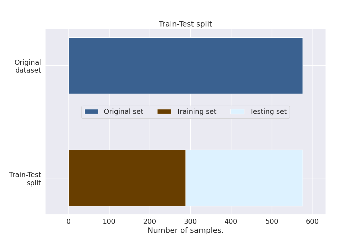
Let’s visualize the first option with a util function.

The following figure illustrates split of entire dataset into the training and testing subsets.

import seaborn as sns
import matplotlib.pyplot as plt
from matplotlib.patches import Patch

sns.set(font_scale=1.5)


def plot_simple_train_test(ax, all_dataset, train_set, test_set):
    """Create a sample plot for training-testing split."""
    bd_cmap = ["#3A6190", "#683E00", "#DDF2FF", "#2196F3"]

    ax.barh("Original\ndataset", len(all_dataset), left=0,
            height=0.5, color=bd_cmap[0])
    ax.barh("Train-Test\nsplit", len(train_set), left=0,
            height=0.5, color=bd_cmap[1])
    ax.barh("Train-Test\nsplit", len(test_set), left=len(train_set),
            height=0.5, color=bd_cmap[2])

    ax.invert_yaxis()
    ax.set(xlabel="Number of samples.", title="Train-Test split")
    ax.legend(["Original set", "Training set", "Testing set"], loc='lower center',
              ncols=4, bbox_to_anchor=(0.5, 0.5))
    ax.set_xlim([-int(0.1 * len(all_dataset)), int(1.1 * len(all_dataset))])
    return ax


fig, ax = plt.subplots(figsize=(12, 8))
plot_simple_train_test(ax=ax, all_dataset=windows_dataset,
                       train_set=train_set, test_set=test_set)

<Axes: title={'center': 'Train-Test split'}, xlabel='Number of samples.'>

Option 2: Train-Val-Test Split

When evaluating different settings hyperparameters for your model, there is still a risk of overfitting on the test set because the parameters can be tweaked until the estimator performs optimally. For more information visit sklearns Cross-Validation Guide. This second option splits the original train_set into two distinct sets, the training set and the validation set to avoid overfitting the hyperparameters to the test set.

Note

If your dataset is really small, the validation split can become quite small. This may lead to unreliable tuning results. To avoid this, either use Option 3 or adjust the split ratio.

To split the train_set we will make use of the train_split argument of EEGClassifier. If you leave this empty (not None!), skorch will make an 80-20 train-validation split. If you want to control the split manually you can do that by using Subset from torch and predefined_split from skorch.

from torch.utils.data import Subset
from sklearn.model_selection import train_test_split
from skorch.helper import predefined_split, SliceDataset

X_train = SliceDataset(train_set, idx=0)
y_train = np.array([y for y in SliceDataset(train_set, idx=1)])
train_indices, val_indices = train_test_split(
    X_train.indices_, test_size=0.2, shuffle=False
)
train_subset = Subset(train_set, train_indices)
val_subset = Subset(train_set, val_indices)

Note

The parameter shuffle is set to False. For time-series data this should always be the case as shuffling might take advantage of correlated samples, which would make the validation performance less meaningful.

clf = EEGClassifier(
    model,
    criterion=torch.nn.NLLLoss,
    optimizer=torch.optim.AdamW,
    train_split=predefined_split(val_subset),
    optimizer__lr=lr,
    optimizer__weight_decay=weight_decay,
    batch_size=batch_size,
    callbacks=[
        "accuracy",
        ("lr_scheduler", LRScheduler("CosineAnnealingLR", T_max=n_epochs - 1)),
    ],
    device=device,
    classes=classes,
    max_epochs=n_epochs,
)
clf.fit(train_subset, y=None)

# evaluate the model after training and validation
y_test = test_set.get_metadata().target
test_acc = clf.score(test_set, y=y_test)
print(f"Test acc: {(test_acc * 100):.2f}%")

  epoch    train_accuracy    train_loss    valid_acc    valid_accuracy    valid_loss      lr     dur
-------  ----------------  ------------  -----------  ----------------  ------------  ------  ------
      1            0.3435        1.3505       0.2759            0.2759        2.2666  0.0006  0.9979
      2            0.3478        1.1789       0.2759            0.2759        2.0685  0.0000  0.9027
Test acc: 27.43%

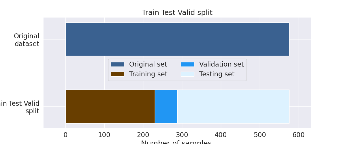
Let’s visualize the second option with a util function.

The following figure illustrates split of entire dataset into the training, validation and testing subsets. Making more compact plot_train_valid_test function.

def plot_train_valid_test(ax, all_dataset, train_subset, val_subset, test_set):
    """Create a sample plot for training, validation, testing."""

    bd_cmap = ["#3A6190", "#683E00", "#2196F3", "#DDF2FF", ]

    n_train, n_val, n_test = len(train_subset), len(val_subset), len(test_set)
    ax.barh("Original\ndataset", len(all_dataset), left=0, height=0.5, color=bd_cmap[0])
    ax.barh("Train-Test-Valid\nsplit", n_train, left=0, height=0.5, color=bd_cmap[1])
    ax.barh("Train-Test-Valid\nsplit", n_val, left=n_train, height=0.5, color=bd_cmap[2])
    ax.barh("Train-Test-Valid\nsplit", n_test, left=n_train + n_val, height=0.5, color=bd_cmap[3])

    ax.invert_yaxis()
    ax.set(xlabel="Number of samples.", title="Train-Test-Valid split")
    ax.legend(["Original set", "Training set", "Validation set", "Testing set"],
              loc="lower center", ncols=2, bbox_to_anchor=(0.5, 0.4))
    ax.set_xlim([-int(0.1 * len(all_dataset)), int(1.1 * len(all_dataset))])
    return ax


fig, ax = plt.subplots(figsize=(12, 5))
plot_train_valid_test(ax=ax, all_dataset=windows_dataset,
                      train_subset=train_subset, val_subset=val_subset, test_set=test_set,)

<Axes: title={'center': 'Train-Test-Valid split'}, xlabel='Number of samples.'>

Option 3: k-Fold Cross Validation

As mentioned above, using only one validation split might not be sufficient, as there might be a shift in the data distribution. To compensate for this, one can run a k-fold Cross Validation, where every sample of the training set is in the validation set once. After averaging over the k validation scores afterwards, you get a very reliable estimate of how the model would perform on unseen data (test set).

Note

This k-Fold Cross Validation can be used without a separate (holdout) test set. If there is no test set available, e.g. in a competition, this scheme is highly recommended to get a reliable estimate of the generalization performance.

To implement this, we will make use of sklearn function cross_val_score and the KFold. CV splitter. The train_split argument has to be set to None, as sklearn will take care of the splitting.

from skorch.callbacks import LRScheduler

from braindecode import EEGClassifier

from sklearn.model_selection import KFold, cross_val_score

lr = 0.0625 * 0.01
weight_decay = 0
batch_size = 64
n_epochs = 2

clf = EEGClassifier(
    model,
    criterion=torch.nn.NLLLoss,
    optimizer=torch.optim.AdamW,
    train_split=None,
    optimizer__lr=lr,
    optimizer__weight_decay=weight_decay,
    batch_size=batch_size,
    callbacks=[
        "accuracy",
        ("lr_scheduler", LRScheduler("CosineAnnealingLR", T_max=n_epochs - 1)),
    ],
    device=device,
    classes=classes,
    max_epochs=n_epochs,
)

train_val_split = KFold(n_splits=5, shuffle=False)
# By setting n_jobs=-1, cross-validation is performed
# with all the processors, in this case the output of the training
# process is not printed sequentially
cv_results = cross_val_score(
    clf, X_train, y_train, scoring="accuracy", cv=train_val_split, n_jobs=1
)
print(
    f"Validation accuracy: {np.mean(cv_results * 100):.2f}"
    f"+-{np.std(cv_results * 100):.2f}%"
)

  epoch    train_accuracy    train_loss      lr     dur
-------  ----------------  ------------  ------  ------
      1            0.3870        1.2082  0.0006  0.9258
      2            0.3957        1.1560  0.0000  0.8180
  epoch    train_accuracy    train_loss      lr     dur
-------  ----------------  ------------  ------  ------
      1            0.2870        1.2641  0.0006  0.8551
      2            0.2870        1.2266  0.0000  0.8161
  epoch    train_accuracy    train_loss      lr     dur
-------  ----------------  ------------  ------  ------
      1            0.4000        1.3003  0.0006  0.8396
      2            0.4087        1.1477  0.0000  0.8394
  epoch    train_accuracy    train_loss      lr     dur
-------  ----------------  ------------  ------  ------
      1            0.2727        1.2076  0.0006  0.8392
      2            0.2900        1.1233  0.0000  0.8413
  epoch    train_accuracy    train_loss      lr     dur
-------  ----------------  ------------  ------  ------
      1            0.4242        1.1577  0.0006  0.8404
      2            0.4286        1.0504  0.0000  0.8377
Validation accuracy: 31.94+-5.59%

Let’s visualize the third option with a util function.

def plot_k_fold(ax, cv, all_dataset, X_train, y_train, test_set):
    """Create a sample plot for training, validation, testing."""

    bd_cmap = ["#3A6190", "#683E00", "#2196F3", "#DDF2FF", ]

    ax.barh("Original\nDataset", len(all_dataset), left=0, height=0.5, color=bd_cmap[0])

    # Generate the training/validation/testing data fraction visualizations for each CV split
    for ii, (tr_idx, val_idx) in enumerate(cv.split(X=X_train, y=y_train)):
        n_train, n_val, n_test = len(tr_idx), len(val_idx), len(test_set)
        n_train2 = n_train + n_val - max(val_idx) - 1
        ax.barh("cv" + str(ii + 1), min(val_idx), left=0, height=0.5, color=bd_cmap[1])
        ax.barh("cv" + str(ii + 1), n_val, left=min(val_idx), height=0.5, color=bd_cmap[2])
        ax.barh("cv" + str(ii + 1), n_train2, left=max(val_idx) + 1, height=0.5, color=bd_cmap[1])
        ax.barh("cv" + str(ii + 1), n_test, left=n_train + n_val, height=0.5, color=bd_cmap[3])

    ax.invert_yaxis()
    ax.set_xlim([-int(0.1 * len(all_dataset)), int(1.1 * len(all_dataset))])
    ax.set(xlabel="Number of samples.", title="KFold Train-Test-Valid split")
    ax.legend([Patch(color=bd_cmap[i]) for i in range(4)],
              ["Original set", "Training set", "Validation set", "Testing set"],
              loc="lower center", ncols=2)
    ax.text(-0.07, 0.45, 'Train-Valid-Test split', rotation=90,
            verticalalignment='center', horizontalalignment='left', transform=ax.transAxes)
    return ax


fig, ax = plt.subplots(figsize=(15, 7))
plot_k_fold(ax, cv=train_val_split, all_dataset=windows_dataset,
            X_train=X_train, y_train=y_train, test_set=test_set,)

<Axes: title={'center': 'KFold Train-Test-Valid split'}, xlabel='Number of samples.'>

How to tune your hyperparameters

One way to do hyperparameter tuning is to run each configuration manually (via Option 2 or 3 from above) and compare the validation performance afterwards. In the early stages of your development process this might be sufficient to get a rough understanding of how your hyperparameter should look like for your model to converge. However, this manual tuning process quickly becomes messy as the number of hyperparameters you want to (jointly) tune increases. Therefore you should, automate this process. We will present two different options, analogous to Option 2 and 3 from above.

Option 1: Train-Val-Test Split

We will again make use of the sklearn library to do the hyperparameter search. GridSearchCV will perform a Grid Search over the parameters specified in param_grid. We use grid search for the model selection as a simple example, but you can use other strategies as well. (List of the sklearn classes for model selection.)

import pandas as pd
from sklearn.model_selection import GridSearchCV

train_val_split = [
    tuple(train_test_split(X_train.indices_, test_size=0.2, shuffle=False))
]

param_grid = {
    "optimizer__lr": [0.00625, 0.000625],
}

# By setting n_jobs=-1, grid search is performed
# with all the processors, in this case the output of the training
# process is not printed sequentially
search = GridSearchCV(
    estimator=clf,
    param_grid=param_grid,
    cv=train_val_split,
    return_train_score=True,
    scoring="accuracy",
    refit=True,
    verbose=1,
    error_score="raise",
    n_jobs=1,
)

search.fit(X_train, y_train)
search_results = pd.DataFrame(search.cv_results_)

best_run = search_results[search_results["rank_test_score"] == 1].squeeze()

best_parameters = best_run["params"]

Fitting 1 folds for each of 2 candidates, totalling 2 fits
  epoch    train_accuracy    train_loss      lr     dur
-------  ----------------  ------------  ------  ------
      1            0.2826        1.5258  0.0063  0.9229
      2            0.4000        1.4053  0.0000  0.8381
  epoch    train_accuracy    train_loss      lr     dur
-------  ----------------  ------------  ------  ------
      1            0.4826        1.2205  0.0006  0.8599
      2            0.5130        1.1218  0.0000  0.8271
  epoch    train_accuracy    train_loss      lr     dur
-------  ----------------  ------------  ------  ------
      1            0.4375        1.2991  0.0006  1.1781
      2            0.4688        1.1161  0.0000  1.1094

Option 2: k-Fold Cross Validation

To perform a full k-Fold CV just replace train_val_split from above with the KFold cross-validator from sklearn.

train_val_split = KFold(n_splits=5, shuffle=False)

References

[1] (1,2)

Tangermann, M., Müller, K.R., Aertsen, A., Birbaumer, N., Braun, C., Brunner, C., Leeb, R., Mehring, C., Miller, K.J., Mueller-Putz, G. and Nolte, G., 2012. Review of the BCI competition IV. Frontiers in neuroscience, 6, p.55.

[2]

Jayaram, Vinay, and Alexandre Barachant. “MOABB: trustworthy algorithm benchmarking for BCIs.” Journal of neural engineering 15.6 (2018): 066011.

[3]

Schirrmeister, R.T., Springenberg, J.T., Fiederer, L.D.J., Glasstetter, M., Eggensperger, K., Tangermann, M., Hutter, F., Burgard, W. and Ball, T. (2017), Deep learning with convolutional neural networks for EEG decoding and visualization. Hum. Brain Mapping, 38: 5391-5420. https://doi.org/10.1002/hbm.23730.

Estimated memory usage: 280 MB