
Note
Go to the end to download the full example code.
Data Augmentation on BCIC IV 2a Dataset#
This tutorial shows how to train EEG deep models with data augmentation. It follows the trial-wise decoding example and also illustrates the effect of a transform on the input signals.
# Authors: Simon Brandt <simonbrandt@protonmail.com>
#          Cédric Rommel <cedric.rommel@inria.fr>
#
# License: BSD (3-clause)
Loading and preprocessing the dataset#
Loading#
from skorch.callbacks import LRScheduler
from skorch.helper import predefined_split

from braindecode import EEGClassifier
from braindecode.datasets import MOABBDataset

subject_id = 3
dataset = MOABBDataset(dataset_name="BNCI2014_001", subject_ids=[subject_id])
Preprocessing#
from numpy import multiply

from braindecode.preprocessing import (
    Preprocessor,
    exponential_moving_standardize,
    preprocess,
)

low_cut_hz = 4.0  # low cut frequency for filtering
high_cut_hz = 38.0  # high cut frequency for filtering
# Parameters for exponential moving standardization
factor_new = 1e-3
init_block_size = 1000
# Factor to convert from V to uV
factor = 1e6

preprocessors = [
    Preprocessor("pick_types", eeg=True, meg=False, stim=False),  # Keep EEG sensors
    Preprocessor(lambda data: multiply(data, factor)),  # Convert from V to uV
    Preprocessor("filter", l_freq=low_cut_hz, h_freq=high_cut_hz),  # Bandpass filter
    Preprocessor(
        exponential_moving_standardize,  # Exponential moving standardization
        factor_new=factor_new,
        init_block_size=init_block_size,
    ),
]

preprocess(dataset, preprocessors, n_jobs=-1)
Extracting windows#
from braindecode.preprocessing import create_windows_from_events

trial_start_offset_seconds = -0.5
# Extract sampling frequency, check that they are same in all datasets
sfreq = dataset.datasets[0].raw.info["sfreq"]
assert all([ds.raw.info["sfreq"] == sfreq for ds in dataset.datasets])
# Calculate the trial start offset in samples.
trial_start_offset_samples = int(trial_start_offset_seconds * sfreq)

# Create windows using braindecode function for this. It needs parameters to
# define how trials should be used.
windows_dataset = create_windows_from_events(
    dataset,
    trial_start_offset_samples=trial_start_offset_samples,
    trial_stop_offset_samples=0,
    preload=True,
)
Split dataset into train and valid#
Defining a Transform#
Data can be manipulated by transforms, which are callable objects. A transform is usually handled by a custom data loader, but can also be called directly on input data, as demonstrated below for illutrative purposes.
First, we need to define a Transform. Here we chose the FrequencyShift, which randomly translates all frequencies within a given range.
from braindecode.augmentation import FrequencyShift

transform = FrequencyShift(
    probability=1.0,  # defines the probability of actually modifying the input
    sfreq=sfreq,
    max_delta_freq=2.0,  # the frequency shifts are sampled now between -2 and 2 Hz
)
Manipulating one session and visualizing the transformed data#
Next, let us augment one session to show the resulting frequency shift. The data of an mne Epoch is used here to make usage of mne functions.
import numpy as np
import torch

X = np.stack([X for X, y, i in train_set.datasets[0]])
# This allows to apply the transform with a fixed shift (10 Hz) for
# visualization instead of sampling the shift randomly between -2 and 2 Hz
X_tr, _ = transform.operation(torch.as_tensor(X).float(), None, 10.0, sfreq)  # type: ignore[has-type]
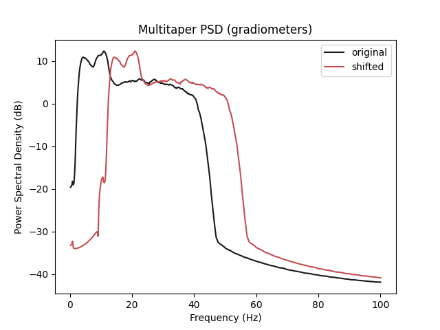
The psd of the transformed session has now been shifted by 10 Hz, as one can see on the psd plot.
import matplotlib.pyplot as plt
import mne


def plot_psd(data, axis, label, color):
    psds, freqs = mne.time_frequency.psd_array_multitaper(
        data, sfreq=sfreq, fmin=0.1, fmax=100
    )
    psds = 10.0 * np.log10(psds)
    psds_mean = psds.mean(0).mean(0)
    axis.plot(freqs, psds_mean, color=color, label=label)


_, ax = plt.subplots()
plot_psd(X, ax, "original", "k")
plot_psd(X_tr.numpy(), ax, "shifted", "r")

ax.set(
    title="Multitaper PSD (gradiometers)",
    xlabel="Frequency (Hz)",
    ylabel="Power Spectral Density (dB)",
)
ax.legend()
plt.show()
Training a model with data augmentation#
Now that we know how to instantiate Transforms, it is time to learn how
to use them to train a model and try to improve its generalization power.
Let’s first create a model.
Create model#
The model to be trained is defined as usual.
from braindecode.models import ShallowFBCSPNet
from braindecode.util import set_random_seeds

cuda = torch.cuda.is_available()  # check if GPU is available, if True chooses to use it
device = "cuda" if cuda else "cpu"
if cuda:
    torch.backends.cudnn.benchmark = True

# Set random seed to be able to roughly reproduce results
# Note that with cudnn benchmark set to True, GPU indeterminism
# may still make results substantially different between runs.
# To obtain more consistent results at the cost of increased computation time,
# you can set `cudnn_benchmark=False` in `set_random_seeds`
# or remove `torch.backends.cudnn.benchmark = True`
seed = 20200220
set_random_seeds(seed=seed, cuda=cuda)

n_classes = 4
classes = list(range(n_classes))

# Extract number of chans and time steps from dataset
n_channels = train_set[0][0].shape[0]
n_times = train_set[0][0].shape[1]

model = ShallowFBCSPNet(
    n_chans=n_channels,
    n_outputs=n_classes,
    n_times=n_times,
    final_conv_length="auto",
)
Create an EEGClassifier with the desired augmentation#
In order to train with data augmentation, a custom data loader can be
for the training. Multiple transforms can be passed to it and will be applied
sequentially to the batched data within the AugmentedDataLoader object.
from braindecode.augmentation import AugmentedDataLoader, SignFlip

freq_shift = FrequencyShift(
    probability=0.5,
    sfreq=sfreq,
    max_delta_freq=2.0,  # the frequency shifts are sampled now between -2 and 2 Hz
)

sign_flip = SignFlip(probability=0.1)

transforms = [freq_shift, sign_flip]

# Send model to GPU
if cuda:
    model.cuda()
The model is now trained as in the trial-wise example. The
AugmentedDataLoader is used as the train iterator and the list of
transforms are passed as arguments.
lr = 0.0625 * 0.01
weight_decay = 0

batch_size = 64
n_epochs = 4

clf = EEGClassifier(
    model,
    iterator_train=AugmentedDataLoader,  # This tells EEGClassifier to use a custom DataLoader
    iterator_train__transforms=transforms,  # This sets the augmentations to use
    criterion=torch.nn.CrossEntropyLoss,
    optimizer=torch.optim.AdamW,
    train_split=predefined_split(valid_set),  # using valid_set for validation
    optimizer__lr=lr,
    optimizer__weight_decay=weight_decay,
    batch_size=batch_size,
    callbacks=[
        "accuracy",
        ("lr_scheduler", LRScheduler("CosineAnnealingLR", T_max=n_epochs - 1)),
    ],
    device=device,
    classes=classes,
)
# Model training for a specified number of epochs. `y` is None as it is already
# supplied in the dataset.
clf.fit(train_set, y=None, epochs=n_epochs)
  epoch    train_accuracy    train_loss    valid_acc    valid_accuracy    valid_loss      lr     dur
-------  ----------------  ------------  -----------  ----------------  ------------  ------  ------
      1            0.2500        1.5869       0.2500            0.2500        6.2989  0.0006  2.1816
      2            0.2500        1.2203       0.2500            0.2500        6.2202  0.0005  1.9788
      3            0.2569        1.1668       0.2431            0.2431        5.2575  0.0002  1.9583
      4            0.2569        1.1553       0.2465            0.2465        4.3377  0.0000  1.9614
Manually composing Transforms#
It would be equivalent (although more verbose) to pass to EEGClassifier a
composition of the same transforms:
from braindecode.augmentation import Compose

composed_transforms = Compose(transforms=transforms)
Setting the data augmentation at the Dataset level#
Also note that it is also possible for most of the transforms to pass them
directly to the WindowsDataset object through the transform argument, as
most commonly done in other libraries. However, it is advised to use the
AugmentedDataLoader as above, as it is compatible with all transforms and
can be more efficient.
Total running time of the script: (0 minutes 28.920 seconds)
Estimated memory usage: 1073 MB
Run this example