Cleaning EEG Data with EEGPrep for Trialwise Decoding

This is a variant of the basic Trialwise decoding tutorial decoding example that additionally inserts an EEGPrep stage into the preprocessing pipeline as a minimal demonstration of how to use EEGPrep with Braindecode.

Loading and preparing the data

Loading the dataset

First, we load the data. In this tutorial, we load the BCI Competition IV 2a data [1] using braindecode’s wrapper to load via MOABB library [2].

Note

To load your own datasets either via mne or from preprocessed X/y numpy arrays, see MNE Dataset Example and Custom Dataset Example.

from braindecode.datasets import MOABBDataset

subject_id = 3
dataset = MOABBDataset(dataset_name="BNCI2014_001", subject_ids=[subject_id])

MNE_DATA is not already configured. It will be set to default location in the home directory - /home/runner/mne_data
All datasets will be downloaded to this location, if anything is already downloaded, please move manually to this location
/opt/hostedtoolcache/Python/3.12.12/x64/lib/python3.12/site-packages/moabb/datasets/download.py:56: RuntimeWarning: Setting non-standard config type: "MNE_DATASETS_BNCI_PATH"
  set_config(key, get_config("MNE_DATA"))

Preprocessing

Now we apply a series of preprocessing steps to our dataset.

The conventional approach in deep learning is to keep preprocessing minimal and leave it to the model to learn relevant features, as done in the seminal early use of deep learning on EEG in [3] and many subsequent works.

However, since EEG can contain quite dramatic artifacts that can easily dwarf the signal of interest and which may harm learning or throw off predictions, additional artifact removal steps can be beneficial in conjunction with deep models. The following code starts from the minimal preprocessing pipeline in Trialwise decoding tutorial and inserts the EEGPrep Preprocessor into the pipeline. This is an integration with the eegprep preprocessing library that implements a series of automated artifact removal steps first proposed in [4] and later refined as part of the (now-default) raw-data preprocessing approach in EEGLAB [5].

The EEGPrep class represents the default end-to-end preprocessing pipeline, which has only a few primary parameters that are worth tuning for a given dataset, the most important ones of which are shown in the code below.

Besides using the end-to-end pipeline as a whole, users can also separately invoke the individual preprocessing steps implemented in EEGPrep as needed; for additional details see the documentation for EEGPrep.

Note

EEGPrep is best used early in the preprocessing pipeline, when you are still acting on continuous (raw) data. The nature of the data after processing is essentially the same as the input (minus many of the artifacts), so you can typically retain most other processing steps that your pipeline would otherwise use, as below.

from numpy import multiply

from braindecode.preprocessing import (
    EEGPrep,
    Preprocessor,
    exponential_moving_standardize,
    preprocess,
)

low_cut_hz = 4.0  # low cut frequency for filtering
high_cut_hz = 38.0  # high cut frequency for filtering
# Parameters for exponential moving standardization
factor_new = 1e-3
init_block_size = 1000
# Factor to convert from V to uV
factor = 1e6

preprocessors = [
    # If you have non-EEG channels in the data that you do not want to keep,
    # it is best to remove them early on, which is more memory-efficient.
    # EEGPrep generally only acts on the EEG channels.
    Preprocessor("pick_types", eeg=True, meg=False, stim=False),
    # This particular dataset requires a conversion from V to uV; this
    # could also be done later in the pipeline since EEGPrep does not
    # care about absolute scaling
    Preprocessor(lambda data: multiply(data, factor)),
    # Here we insert the EEGPrep preprocessing step; experiment with commenting
    # this out to see how it affects results. You can also disable additional
    # processing steps in the pipeline by setting select parameters to None.
    EEGPrep(
        resample_to=128,
        # This is best disabled for single-trial classification (see EEGPrep docs)
        bad_window_max_bad_channels=None,
        # The following examples show some other frequently used non-default values:
        # burst_removal_cutoff=15.0,       # 15.0 -> less aggressive burst removal
        # bad_channel_corr_threshold=0.75, # 0.75 -> less aggressive channel removal
    ),
    Preprocessor("filter", l_freq=low_cut_hz, h_freq=high_cut_hz),  # Bandpass filter
    Preprocessor(
        exponential_moving_standardize,  # Exponential moving standardization
        factor_new=factor_new,
        init_block_size=init_block_size,
    ),
]

# Transform the data
preprocess(dataset, preprocessors, n_jobs=-1)

/home/runner/work/braindecode/braindecode/braindecode/preprocessing/preprocess.py:71: UserWarning: Preprocessing choices with lambda functions cannot be saved.
  warn("Preprocessing choices with lambda functions cannot be saved.")

<braindecode.datasets.moabb.MOABBDataset object at 0x7ff8188638c0>

Besides using the end-to-end pipeline as a whole, you can also separately invoke the individual preprocessing steps implemented in EEGPrep as needed; see the EEGPrep class documentation for details.

Note

When using individual artifact removal steps, make sure they are applied in the intended order, since otherwise you may get suboptimal results.

Extracting Compute Windows

Now we extract compute windows from the signals, these will be the inputs to the deep networks during training. In the case of trialwise decoding, we just have to decide if we want to include some part before and/or after the trial. For our work with this dataset, it was often beneficial to also include the 500 ms before the trial.

from braindecode.preprocessing import create_windows_from_events

trial_start_offset_seconds = -0.5
# Extract sampling frequency, check that they are same in all datasets
sfreq = dataset.datasets[0].raw.info["sfreq"]
assert all([ds.raw.info["sfreq"] == sfreq for ds in dataset.datasets])
# Calculate the trial start offset in samples.
trial_start_offset_samples = int(trial_start_offset_seconds * sfreq)

# Create windows using braindecode function for this. It needs parameters to define how
# trials should be used.
windows_dataset = create_windows_from_events(
    dataset,
    trial_start_offset_samples=trial_start_offset_samples,
    trial_stop_offset_samples=0,
    preload=True,
)

Splitting the dataset into training and validation sets

We can easily split the dataset using additional info stored in the description attribute, in this case session column. We select 0train for training and 1test for validation.

splitted = windows_dataset.split("session")
train_set = splitted["0train"]  # Session train
valid_set = splitted["1test"]  # Session evaluation

Creating a model

Now we create the deep learning model! Braindecode comes with some predefined convolutional neural network architectures for raw time-domain EEG. Here, we use the EEGNet model from [6]. These models are pure PyTorch deep learning models, therefore to use your own model, it just has to be a normal PyTorch torch.nn.Module.

import torch

from braindecode.models import EEGNet
from braindecode.util import set_random_seeds

cuda = torch.cuda.is_available()  # check if GPU is available, if True chooses to use it
device = "cuda" if cuda else "cpu"
if cuda:
    torch.backends.cudnn.benchmark = True
# Set random seed to be able to roughly reproduce results
# Note that with cudnn benchmark set to True, GPU indeterminism
# may still make results substantially different between runs.
# To obtain more consistent results at the cost of increased computation time,
# you can set `cudnn_benchmark=False` in `set_random_seeds`
# or remove `torch.backends.cudnn.benchmark = True`
seed = 20200220
set_random_seeds(seed=seed, cuda=cuda)

n_classes = 4
classes = list(range(n_classes))
# Extract number of chans and time steps from dataset
n_chans = train_set[0][0].shape[0]
n_times = train_set[0][0].shape[1]

# EEGNet is a pretty strong default pick for a variety of tasks, but
# be sure to review the tuning parameters, which may not be optimal for your
# task out of the box.
model = EEGNet(
    n_chans,
    n_classes,
    n_times=n_times,
)

# Display torchinfo table describing the model
print(model)

# Send model to GPU
if cuda:
    model = model.cuda()

================================================================================================================================================================
Layer (type (var_name):depth-idx)                            Input Shape               Output Shape              Param #                   Kernel Shape
================================================================================================================================================================
EEGNet (EEGNet)                                              [1, 22, 65]               [1, 4]                    --                        --
├─Ensure4d (ensuredims): 1-1                                 [1, 22, 65]               [1, 22, 65, 1]            --                        --
├─Rearrange (dimshuffle): 1-2                                [1, 22, 65, 1]            [1, 1, 22, 65]            --                        --
├─Conv2d (conv_temporal): 1-3                                [1, 1, 22, 65]            [1, 8, 22, 66]            512                       [1, 64]
├─BatchNorm2d (bnorm_temporal): 1-4                          [1, 8, 22, 66]            [1, 8, 22, 66]            16                        --
├─ParametrizedConv2dWithConstraint (conv_spatial): 1-5       [1, 8, 22, 66]            [1, 16, 1, 66]            --                        [22, 1]
│    └─ModuleDict (parametrizations): 2-1                    --                        --                        --                        --
│    │    └─ParametrizationList (weight): 3-1                --                        [16, 1, 22, 1]            352                       --
├─BatchNorm2d (bnorm_1): 1-6                                 [1, 16, 1, 66]            [1, 16, 1, 66]            32                        --
├─ELU (elu_1): 1-7                                           [1, 16, 1, 66]            [1, 16, 1, 66]            --                        --
├─AvgPool2d (pool_1): 1-8                                    [1, 16, 1, 66]            [1, 16, 1, 16]            --                        [1, 4]
├─Dropout (drop_1): 1-9                                      [1, 16, 1, 16]            [1, 16, 1, 16]            --                        --
├─Conv2d (conv_separable_depth): 1-10                        [1, 16, 1, 16]            [1, 16, 1, 17]            256                       [1, 16]
├─Conv2d (conv_separable_point): 1-11                        [1, 16, 1, 17]            [1, 16, 1, 17]            256                       [1, 1]
├─BatchNorm2d (bnorm_2): 1-12                                [1, 16, 1, 17]            [1, 16, 1, 17]            32                        --
├─ELU (elu_2): 1-13                                          [1, 16, 1, 17]            [1, 16, 1, 17]            --                        --
├─AvgPool2d (pool_2): 1-14                                   [1, 16, 1, 17]            [1, 16, 1, 2]             --                        [1, 8]
├─Dropout (drop_2): 1-15                                     [1, 16, 1, 2]             [1, 16, 1, 2]             --                        --
├─Sequential (final_layer): 1-16                             [1, 16, 1, 2]             [1, 4]                    --                        --
│    └─Conv2d (conv_classifier): 2-2                         [1, 16, 1, 2]             [1, 4, 1, 1]              132                       [1, 2]
│    └─Rearrange (permute_back): 2-3                         [1, 4, 1, 1]              [1, 4, 1, 1]              --                        --
│    └─SqueezeFinalOutput (squeeze): 2-4                     [1, 4, 1, 1]              [1, 4]                    --                        --
│    │    └─Rearrange (squeeze): 3-2                         [1, 4, 1, 1]              [1, 4, 1]                 --                        --
================================================================================================================================================================
Total params: 1,588
Trainable params: 1,588
Non-trainable params: 0
Total mult-adds (Units.MEGABYTES): 0.75
================================================================================================================================================================
Input size (MB): 0.01
Forward/backward pass size (MB): 0.20
Params size (MB): 0.00
Estimated Total Size (MB): 0.21
================================================================================================================================================================

Model Training

Now we will train the network! EEGClassifier is a Braindecode object responsible for managing the training of neural networks. It inherits from skorch.classifier.NeuralNetClassifier, so the training logic is the same as in skorch.

Note

In this tutorial, we use some default parameters that we have found to work well for motor decoding, however we strongly encourage you to perform your own hyperparameter optimization using cross validation on your training data.

from skorch.callbacks import LRScheduler
from skorch.helper import predefined_split

from braindecode import EEGClassifier

# We found these values to be good for the shallow network:
lr = 0.0625 * 0.01
weight_decay = 0

# For deep4 they should be:
# lr = 1 * 0.01
# weight_decay = 0.5 * 0.001

batch_size = 64
n_epochs = 4

clf = EEGClassifier(
    model,
    criterion=torch.nn.CrossEntropyLoss,
    optimizer=torch.optim.AdamW,
    train_split=predefined_split(valid_set),  # using valid_set for validation
    optimizer__lr=lr,
    optimizer__weight_decay=weight_decay,
    batch_size=batch_size,
    callbacks=[
        "accuracy",
        ("lr_scheduler", LRScheduler("CosineAnnealingLR", T_max=n_epochs - 1)),
    ],
    device=device,
    classes=classes,
)
# Model training for the specified number of epochs. ``y`` is ``None`` as it is
# already supplied in the dataset.
_ = clf.fit(train_set, y=None, epochs=n_epochs)

  epoch    train_accuracy    train_loss    valid_acc    valid_accuracy    valid_loss      lr     dur
-------  ----------------  ------------  -----------  ----------------  ------------  ------  ------
      1            0.2639        1.4037       0.2361            0.2361        1.3863  0.0006  0.1257
      2            0.2569        1.3936       0.2535            0.2535        1.3863  0.0005  0.1041
      3            0.2569        1.3856       0.2465            0.2465        1.3863  0.0002  0.1041
      4            0.2535        1.3953       0.2396            0.2396        1.3863  0.0000  0.1042

Plotting Results

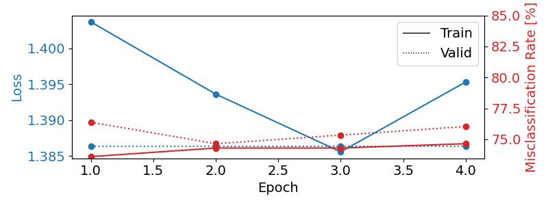
Now we use the history stored by skorch throughout training to plot accuracy and loss curves.

import matplotlib.pyplot as plt
import pandas as pd
from matplotlib.lines import Line2D

# Extract loss and accuracy values for plotting from history object
results_columns = ["train_loss", "valid_loss", "train_accuracy", "valid_accuracy"]
df = pd.DataFrame(
    clf.history[:, results_columns],
    columns=results_columns,
    index=clf.history[:, "epoch"],
)

# get percent of misclass for better visual comparison to loss
df = df.assign(
    train_misclass=100 - 100 * df.train_accuracy,
    valid_misclass=100 - 100 * df.valid_accuracy,
)

fig, ax1 = plt.subplots(figsize=(8, 3))
df.loc[:, ["train_loss", "valid_loss"]].plot(
    ax=ax1, style=["-", ":"], marker="o", color="tab:blue", legend=False, fontsize=14
)

ax1.tick_params(axis="y", labelcolor="tab:blue", labelsize=14)
ax1.set_ylabel("Loss", color="tab:blue", fontsize=14)

ax2 = ax1.twinx()  # instantiate a second axes that shares the same x-axis

df.loc[:, ["train_misclass", "valid_misclass"]].plot(
    ax=ax2, style=["-", ":"], marker="o", color="tab:red", legend=False
)
ax2.tick_params(axis="y", labelcolor="tab:red", labelsize=14)
ax2.set_ylabel("Misclassification Rate [%]", color="tab:red", fontsize=14)
ax2.set_ylim(ax2.get_ylim()[0], 85)  # make some room for legend
ax1.set_xlabel("Epoch", fontsize=14)

# where some data has already been plotted to ax
handles = []
handles.append(
    Line2D([0], [0], color="black", linewidth=1, linestyle="-", label="Train")
)
handles.append(
    Line2D([0], [0], color="black", linewidth=1, linestyle=":", label="Valid")
)
plt.legend(handles, [h.get_label() for h in handles], fontsize=14)
plt.tight_layout()

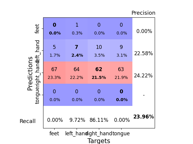
Plotting a Confusion Matrix

Here we generate a confusion matrix as in [3].

from sklearn.metrics import confusion_matrix

from braindecode.visualization import plot_confusion_matrix

# generate confusion matrices
# get the targets
y_true = valid_set.get_metadata().target
y_pred = clf.predict(valid_set)

# generating confusion matrix
confusion_mat = confusion_matrix(y_true, y_pred)

# add class labels
# label_dict is class_name : str -> i_class : int
label_dict = windows_dataset.datasets[0].window_kwargs[0][1]["mapping"]
# sort the labels by values (values are integer class labels)
labels = [k for k, v in sorted(label_dict.items(), key=lambda kv: kv[1])]

# plot the basic conf. matrix
plot_confusion_matrix(confusion_mat, class_names=labels)

<Figure size 640x480 with 1 Axes>

References

[1]

Tangermann, M., Müller, K.R., Aertsen, A., Birbaumer, N., Braun, C., Brunner, C., Leeb, R., Mehring, C., Miller, K.J., Mueller-Putz, G. and Nolte, G., 2012. Review of the BCI competition IV. Frontiers in neuroscience, 6, p.55.

[2]

Jayaram, Vinay, and Alexandre Barachant. “MOABB: trustworthy algorithm benchmarking for BCIs.” Journal of neural engineering 15.6 (2018): 066011.

[3] (1,2)

Schirrmeister, R.T., Springenberg, J.T., Fiederer, L.D.J., Glasstetter, M., Eggensperger, K., Tangermann, M., Hutter, F., Burgard, W. and Ball, T. (2017), Deep learning with convolutional neural networks for EEG decoding and visualization. Hum. Brain Mapping, 38: 5391-5420. https://doi.org/10.1002/hbm.23730.

[4]

Mullen, T.R., Kothe, C.A., Chi, Y.M., Ojeda, A., Kerth, T., Makeig, S., Jung, T.P. and Cauwenberghs, G., 2015. Real-time neuroimaging and cognitive monitoring using wearable dry EEG. IEEE Transactions on Biomedical Engineering, 62(11), pp.2553-2567.

[5]

Delorme, A. and Makeig, S., 2004. EEGLAB: an open source toolbox for analysis of single-trial EEG dynamics including independent component analysis. Journal of Neuroscience Methods, 134(1), pp.9-21.

[6]

Lawhern, V. J., Solon, A. J., Waytowich, N. R., Gordon, S. M., Hung, C. P., & Lance, B. J. (2018). EEGNet: a compact convolutional neural network for EEG-based brain–computer interfaces. Journal of Neural Engineering, 15(5), 056013.

Estimated memory usage: 1232 MB