Hyperparameter tuning with scikit-learn

The braindecode provides some compatibility with scikit-learn. This allows us to use scikit-learn functionality to find the best hyperparameters for our model. This is especially useful to tune hyperparameters or parameters for one decoding task or a specific dataset.

Why do you need to tune the neural networks model?

Deep learning models are often sensitive to the choice of hyperparameters and parameters. Hyperparameters are the parameters set before training the model. The hyperparameters determine (1) the capacity of the model, e.g. its depth (the number of layers) and its width (the number of convolutional kernels, sizes of fully connected layers) and (2) the learning process via the choice of optimizer and its learning rate, the number of epochs, the batch size, the choice of non-linearities, the strategies to initialize the learning weights, etc. On the other hand, parameters are learned during training, such as the neural network weights. The choice of these can have a significant impact on the performance of the model. Therefore, it is important to tune these to maximize the discriminative power of the model, in the case of decoding tasks (classification, regression, etc.), such as sleep staging, BCI, pathology detection, etc. We recommend the Deep Learning Tuning Playbook by Google to learn more about hyperparameters and parameters tuning [1].

In this tutorial, we will use the standard decoding approach to show the impact of the learning rate and dropout probability on the model’s performance.

Loading and preprocessing the dataset

Loading

First, we load the data. In this tutorial, we use the functionality of braindecode to load datasets via MOABB [2] to load the BCI Competition IV 2a data [3].

Note

To load your own datasets either via mne or from preprocessed X/y numpy arrays, see MNE Dataset Example and Custom Dataset Example.

from braindecode.datasets.moabb import MOABBDataset

subject_id = 3
dataset = MOABBDataset(dataset_name="BNCI2014001", subject_ids=[subject_id])

Preprocessing

In this example, preprocessing includes signal rescaling, the bandpass filtering (low and high cut-off frequencies are 4 and 38 Hz) and the standardization using the exponential moving mean and variance. You can either apply functions provided by mne.io.Raw or mne.Epochs or apply your own functions, either to the MNE object or the underlying numpy array.

Note

These prepocessings are now directly applied to the loaded data, and not on-the-fly applied as transformations in PyTorch-libraries like torchvision.

from numpy import multiply

from braindecode.preprocessing.preprocess import (
    Preprocessor,
    exponential_moving_standardize,
    preprocess,
)

low_cut_hz = 4.0  # low cut frequency for filtering
high_cut_hz = 38.0  # high cut frequency for filtering
# Parameters for exponential moving standardization
factor_new = 1e-3
init_block_size = 1000
# Factor to convert from V to uV
factor = 1e6

preprocessors = [
    Preprocessor("pick_types", eeg=True, meg=False, stim=False),
    # Keep EEG sensors
    Preprocessor(lambda data: multiply(data, factor)),  # Convert from V to uV
    Preprocessor("filter", l_freq=low_cut_hz, h_freq=high_cut_hz),
    # Bandpass filter
    Preprocessor(
        exponential_moving_standardize,
        # Exponential moving standardization
        factor_new=factor_new,
        init_block_size=init_block_size,
    ),
]

# Preprocess the data
preprocess(dataset, preprocessors, n_jobs=-1)

/home/runner/work/braindecode/braindecode/braindecode/preprocessing/preprocess.py:71: UserWarning: Preprocessing choices with lambda functions cannot be saved.
  warn("Preprocessing choices with lambda functions cannot be saved.")

<braindecode.datasets.moabb.MOABBDataset object at 0x7ff8187ca4e0>

Extraction of the Compute Windows

Extraction of the Windows

Extraction of the trials (windows) from the time series is based on the events inside the dataset. One event is the demarcation of the stimulus or the beginning of the trial. In this example, we want to analyse 0.5 [s] long before the corresponding event and the duration of the event itself. Therefore, we set the trial_start_offset_seconds to -0.5 [s] and the trial_stop_offset_seconds to 0 [s].

We extract from the dataset the sampling frequency, which is the same for all datasets in this case, and we tested it.

Note

The trial_start_offset_seconds and trial_stop_offset_seconds are defined in seconds and need to be converted into samples (multiplication with the sampling frequency), relative to the event. This variable is dataset dependent.

from braindecode.preprocessing.windowers import create_windows_from_events

trial_start_offset_seconds = -0.5
# Extract sampling frequency, check that they are same in all datasets
sfreq = dataset.datasets[0].raw.info["sfreq"]
assert all([ds.raw.info["sfreq"] == sfreq for ds in dataset.datasets])
# Calculate the trial start offset in samples.
trial_start_offset_samples = int(trial_start_offset_seconds * sfreq)

# Create windows using braindecode function for this. It needs parameters to define how
# trials should be used.
windows_dataset = create_windows_from_events(
    dataset,
    trial_start_offset_samples=trial_start_offset_samples,
    trial_stop_offset_samples=0,
    preload=True,
)

Split dataset into train and valid

We can easily split the dataset using additional info stored in the description attribute, in this case session column. We select 0train for training and 1test for evaluation.

splitted = windows_dataset.split("session")
train_set = splitted["0train"]  # Session train
eval_set = splitted["1test"]  # Session evaluation

Create model

Now we create the deep learning model! Braindecode comes with some predefined convolutional neural network architectures for raw time-domain EEG. Here, we use the ShallowFBCSPNet model from Deep learning with convolutional neural networks for EEG decoding and visualization [4]. These models are pure PyTorch deep learning models, therefore to use your own model, it just has to be a normal PyTorch torch.nn.Module.

from functools import partial

import torch

from braindecode.models import ShallowFBCSPNet
from braindecode.util import set_random_seeds

# check if GPU is available, if True chooses to use it
cuda = torch.cuda.is_available()
device = "cuda" if cuda else "cpu"
if cuda:
    torch.backends.cudnn.benchmark = True
seed = 20200220  # random seed to make results reproducible
# Set random seed to be able to reproduce results
set_random_seeds(seed=seed, cuda=cuda)

n_classes = 4
# Extract number of chans and time steps from dataset
n_chans = train_set[0][0].shape[0]
n_times = train_set[0][0].shape[1]

# To analyze the impact of the different parameters inside the torch model, we
# need to create partial initialisations. This is because the
# GridSearchCV of scikit-learn will try to initialize the model with the
# parameters we want to tune. If we do not do this, the GridSearchCV will
# try to initialize the model with the parameters we want to tune but
# without the parameters we do not want to tune. This will result in an
# error.
model = partial(
    ShallowFBCSPNet,
    n_chans=n_chans,
    n_outputs=n_classes,
    n_times=n_times,
    final_conv_length="auto",
)

# Send model to GPU
if cuda and hasattr(model, "cuda"):
    model.cuda()

Training

Now we train the network! EEGClassifier is a Braindecode object responsible for managing the training of neural networks. It inherits from skorch.classifier.NeuralNetClassifier, so the training logic is the same as in skorch.

from skorch.callbacks import LRScheduler
from skorch.dataset import ValidSplit

from braindecode import EEGClassifier

batch_size = 16
n_epochs = 2

clf = EEGClassifier(
    model,
    criterion=torch.nn.CrossEntropyLoss,
    optimizer=torch.optim.AdamW,
    optimizer__lr=[],  # This will be handled by GridSearchCV
    batch_size=batch_size,
    train_split=ValidSplit(0.2, random_state=seed),
    callbacks=[
        "accuracy",
        ("lr_scheduler", LRScheduler("CosineAnnealingLR", T_max=n_epochs - 1)),
    ],
    device=device,
)

We use scikit-learn GridSearchCV to tune hyperparameters. To be able to do this, we slice the braindecode datasets that by default return a 3-tuple to return X and y, respectively.

Note

The KFold object splits the datasets based on their length which corresponds to the number of compute windows. In this (trialwise) example this is fine to do. In a cropped setting this is not advisable since this might split compute windows of a single trial into both train and valid set.

import pandas as pd
from numpy import array
from sklearn.model_selection import GridSearchCV, KFold
from skorch.helper import SliceDataset

train_X = SliceDataset(train_set, idx=0)
train_y = array([y for y in SliceDataset(train_set, idx=1)])
cv = KFold(n_splits=2, shuffle=True, random_state=42)

learning_rates = [0.00625, 0.0000625]
drop_probs = [0.2, 0.5, 0.8]

fit_params = {"epochs": n_epochs}
param_grid = {"optimizer__lr": learning_rates, "module__drop_prob": drop_probs}

# By setting n_jobs=-1, grid search is performed
# with all the processors, in this case the output of the training
# process is not printed sequentially
search = GridSearchCV(
    estimator=clf,
    param_grid=param_grid,
    cv=cv,
    return_train_score=True,
    scoring="accuracy",
    refit=True,
    verbose=1,
    error_score="raise",
    n_jobs=1,
)

search.fit(train_X, train_y, **fit_params)

# Extract the results into a DataFrame
search_results = pd.DataFrame(search.cv_results_)

Fitting 2 folds for each of 6 candidates, totalling 12 fits
  epoch    train_accuracy    train_loss    valid_acc    valid_accuracy    valid_loss      lr     dur
-------  ----------------  ------------  -----------  ----------------  ------------  ------  ------
      1            0.3217        1.8104       0.3793            0.3793        4.4646  0.0063  0.6553
      2            0.5043        0.8677       0.5862            0.5862        1.7216  0.0000  0.6323
  epoch    train_accuracy    train_loss    valid_acc    valid_accuracy    valid_loss      lr     dur
-------  ----------------  ------------  -----------  ----------------  ------------  ------  ------
      1            0.5217        2.0880       0.5517            0.5517        2.0215  0.0063  0.6288
      2            0.6174        1.0315       0.5172            0.5172        2.0105  0.0000  0.6265
  epoch    train_accuracy    train_loss    valid_acc    valid_accuracy    valid_loss      lr     dur
-------  ----------------  ------------  -----------  ----------------  ------------  ------  ------
      1            0.2783        1.4649       0.0690            0.0690        6.8550  0.0001  0.6182
      2            0.2783        1.4538       0.0690            0.0690        5.1283  0.0000  0.6305
  epoch    train_accuracy    train_loss    valid_acc    valid_accuracy    valid_loss      lr     dur
-------  ----------------  ------------  -----------  ----------------  ------------  ------  ------
      1            0.2000        1.5902       0.3103            0.3103        3.0387  0.0001  0.6245
      2            0.2000        1.4941       0.3103            0.3103        2.4941  0.0000  0.6263
  epoch    train_accuracy    train_loss    valid_acc    valid_accuracy    valid_loss      lr     dur
-------  ----------------  ------------  -----------  ----------------  ------------  ------  ------
      1            0.4087        1.5979       0.3448            0.3448        3.7528  0.0063  0.6211
      2            0.5391        1.0078       0.4138            0.4138        2.0379  0.0000  0.6211
  epoch    train_accuracy    train_loss    valid_acc    valid_accuracy    valid_loss      lr     dur
-------  ----------------  ------------  -----------  ----------------  ------------  ------  ------
      1            0.3043        1.9618       0.3793            0.3793        4.7374  0.0063  0.6282
      2            0.5130        1.6277       0.4138            0.4138        3.2027  0.0000  0.6262
  epoch    train_accuracy    train_loss    valid_acc    valid_accuracy    valid_loss      lr     dur
-------  ----------------  ------------  -----------  ----------------  ------------  ------  ------
      1            0.2783        1.5895       0.0690            0.0690        5.1442  0.0001  0.6256
      2            0.2783        1.6594       0.0690            0.0690        3.9613  0.0000  0.6249
  epoch    train_accuracy    train_loss    valid_acc    valid_accuracy    valid_loss      lr     dur
-------  ----------------  ------------  -----------  ----------------  ------------  ------  ------
      1            0.2783        1.4882       0.2069            0.2069        5.0953  0.0001  0.6251
      2            0.2783        1.4685       0.2069            0.2069        4.0790  0.0000  0.6265
  epoch    train_accuracy    train_loss    valid_acc    valid_accuracy    valid_loss      lr     dur
-------  ----------------  ------------  -----------  ----------------  ------------  ------  ------
      1            0.3217        2.4903       0.4138            0.4138        3.1864  0.0063  0.6175
      2            0.4261        1.7236       0.4138            0.4138        1.5802  0.0000  0.6260
  epoch    train_accuracy    train_loss    valid_acc    valid_accuracy    valid_loss      lr     dur
-------  ----------------  ------------  -----------  ----------------  ------------  ------  ------
      1            0.2435        2.2631       0.3448            0.3448        6.4558  0.0063  0.6248
      2            0.3565        1.4870       0.4483            0.4483        2.6188  0.0000  0.6211
  epoch    train_accuracy    train_loss    valid_acc    valid_accuracy    valid_loss      lr     dur
-------  ----------------  ------------  -----------  ----------------  ------------  ------  ------
      1            0.2609        1.8435       0.0690            0.0690        3.5460  0.0001  0.6157
      2            0.2261        1.7590       0.2069            0.2069        3.0455  0.0000  0.6255
  epoch    train_accuracy    train_loss    valid_acc    valid_accuracy    valid_loss      lr     dur
-------  ----------------  ------------  -----------  ----------------  ------------  ------  ------
      1            0.2609        1.7889       0.2414            0.2414        4.0269  0.0001  0.6160
      2            0.2696        2.0504       0.2414            0.2414        3.2738  0.0000  0.6237
  epoch    train_accuracy    train_loss    valid_acc    valid_accuracy    valid_loss      lr     dur
-------  ----------------  ------------  -----------  ----------------  ------------  ------  ------
      1            0.3261        2.2354       0.2759            0.2759        4.5460  0.0063  1.2483
      2            0.5391        1.2844       0.4138            0.4138        2.1986  0.0000  1.2481

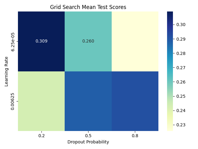
Plotting the results

import matplotlib.pyplot as plt
import seaborn as sns

# Create a pivot table for the heatmap
pivot_table = search_results.pivot(
    index="param_optimizer__lr",
    columns="param_module__drop_prob",
    values="mean_test_score",
)
# Create the heatmap
fig, ax = plt.subplots()
sns.heatmap(pivot_table, annot=True, fmt=".3f", cmap="YlGnBu", cbar=True)
plt.title("Grid Search Mean Test Scores")
plt.ylabel("Learning Rate")
plt.xlabel("Dropout Probability")
plt.tight_layout()
plt.show()

Get the best hyperparameters

best_run = search_results[search_results["rank_test_score"] == 1].squeeze()
print(
    f"Best hyperparameters were {best_run['params']} which gave a validation "
    f"accuracy of {best_run['mean_test_score'] * 100:.2f}% (training "
    f"accuracy of {best_run['mean_train_score'] * 100:.2f}%)."
)

eval_X = SliceDataset(eval_set, idx=0)
eval_y = SliceDataset(eval_set, idx=1)
score = search.score(eval_X, eval_y)
print(f"Eval accuracy is {score * 100:.2f}%.")

Best hyperparameters were {'module__drop_prob': 0.5, 'optimizer__lr': 0.00625} which gave a validation accuracy of 31.60% (training accuracy of 50.35%).
Eval accuracy is 37.15%.

References

[1]

Varun Godbole, George E. Dahl, Justin Gilmer, Christopher J. Shallue, Zachary Nado (2022). Deep Learning Tuning Playbook. Github google-research/tuning_playbook

[2]

Jayaram, Vinay, and Alexandre Barachant. “MOABB: trustworthy algorithm benchmarking for BCIs.” Journal of neural engineering 15.6 (2018): 066011.

[3]

Tangermann, M., Müller, K.R., Aertsen, A., Birbaumer, N., Braun, C., Brunner, C., Leeb, R., Mehring, C., Miller, K.J., Mueller-Putz, G. and Nolte, G., 2012. Review of the BCI competition IV. Frontiers in neuroscience, 6, p.55.

[4]

Schirrmeister, R.T., Springenberg, J.T., Fiederer, L.D.J., Glasstetter, M., Eggensperger, K., Tangermann, M., Hutter, F., Burgard, W. and Ball, T. (2017), Deep learning with convolutional neural networks for EEG decoding and visualization. Hum. Brain Mapping, 38: 5391-5420. https://doi.org/10.1002/hbm.23730.

Estimated memory usage: 1336 MB