Temporal generalization with Braindecode

In this tutorial, we will show you how to use the Braindecode library to decode EEG data over time. The problem of decoding EEG data over time is formulated as fitting a multivariate predictive model on each time point of the signal and then evaluating the performance of the model at the same time point in new epoched data. Specifically, given a pair of features \(X\) and targets \(y\), where \(X\) has more than \(2\) dimensions, we want to fit a model \(f\) to \(X\) and \(y\) and evaluate the performance of \(f\) on a new pair of features \(X'\) and targets \(y'\). Typically, \(X\) is in the shape of \(n_{\text{epochs}} \times n_{\text{channels}} \times n_{\text{time}}\) and \(y\) is in the shape of \(n_{\text{epochs}} \times n_{\text{classes}}\). This tutorial is based on the MNE tutorial: https://mne.tools/stable/auto_tutorials/machine-learning/50_decoding.html#temporal-decoding.

For more information on the problem of temporal generalization, visit MNE [1]. For papers describing this method, see [2] and [3].

Loading and preprocessing the data

We will load in the same exact MEG dataset as used in the MNE tutorial [1] and preprocess it identically.

import matplotlib.pyplot as plt
import mne
import numpy as np
import shap
import torch
import torch.nn as nn
from mne.datasets import sample
from mne.decoding import (
    GeneralizingEstimator,
    SlidingEstimator,
    cross_val_multiscore,
)
from sklearn.pipeline import make_pipeline
from sklearn.preprocessing import LabelEncoder, StandardScaler
from skorch.callbacks import LRScheduler
from torch.optim import AdamW

from braindecode import EEGClassifier
from braindecode.models import EEGSimpleConv

# Configure matplotlib for publication-quality plots
plt.rcParams["figure.figsize"] = (10, 6)
plt.rcParams["font.size"] = 11
plt.rcParams["font.family"] = "sans-serif"
plt.rcParams["axes.linewidth"] = 1.2
plt.rcParams["grid.linewidth"] = 0.8
plt.rcParams["xtick.labelsize"] = 10
plt.rcParams["ytick.labelsize"] = 10
plt.rcParams["axes.labelsize"] = 11
plt.rcParams["legend.fontsize"] = 10
plt.rcParams["figure.titlesize"] = 12
plt.rcParams["axes.spines.left"] = True
plt.rcParams["axes.spines.bottom"] = True
plt.rcParams["axes.spines.top"] = False
plt.rcParams["axes.spines.right"] = False
plt.rcParams["grid.alpha"] = 0.3

device = "cuda" if torch.cuda.is_available() else "cpu"

data_path = sample.data_path()

subjects_dir = data_path / "subjects"
meg_path = data_path / "MEG" / "sample"
raw_fname = meg_path / "sample_audvis_filt-0-40_raw.fif"
tmin, tmax = -0.200, 0.500
event_id = {"Auditory/Left": 1, "Visual/Left": 3}  # just use two
raw = mne.io.read_raw_fif(raw_fname)
raw.pick(picks=["grad", "stim", "eog"])

# The subsequent decoding analyses only capture evoked responses, so we can
# low-pass the MEG data. Usually a value more like 40 Hz would be used,
# but here low-pass at 20 so we can more heavily decimate, and allow
# the example to run faster. The 2 Hz high-pass helps improve CSP.
raw.load_data().filter(2, 20)
events = mne.find_events(raw, "STI 014")

# Set up bad channels (modify to your needs)
raw.info["bads"] += ["MEG 2443"]  # bads + 2 more

# Read epochs
epochs = mne.Epochs(
    raw,
    events,
    event_id,
    tmin,
    tmax,
    proj=True,
    picks=("grad", "eog"),
    baseline=(None, 0.0),
    preload=True,
    reject=dict(grad=4000e-13, eog=150e-6),
    decim=3,
    verbose="error",
)
epochs.pick(picks="meg", exclude="bads")  # remove stim and EOG
del raw

X = epochs.get_data(copy=False)  # MEG signals: n_epochs, n_meg_channels, n_times
y = epochs.events[:, 2]  # target: auditory left vs visual left
y_encod = LabelEncoder().fit_transform(y)
print("X shape: ", X.shape, "Y shape: ", y.shape, "Y encode shape: ", y_encod.shape)

n_classes = len(np.unique(y))
classes = list(range(n_classes))
# Extract number of chans and time steps from dataset
n_chans = X.shape[1]
n_times = X.shape[2]
print(n_classes, classes, n_chans, n_times)

X shape:  (123, 203, 36) Y shape:  (123,) Y encode shape:  (123,)
2 [0, 1] 203 36

Define your model(s)

Unlike the original MNE tutorial, we will use a deep learning model here and leverage the EEGClassifier class from Braindecode. The EEGClassifier class is a wrapper around a PyTorch model that allows us to use the model like a scikit-learn estimator. We define a simple 3 layer multi-layer perceptron (MLP) model with GELU activations:

class BasicMLP(nn.Module):
    """Simple 3 Layer MLP with GELU Activations between first
    and second layer and second and third layers
    """

    def __init__(self, n_chans, n_outputs, n_times):
        super().__init__()
        self.n_chans = n_chans
        self.n_classes = n_outputs
        self.n_times = n_times

        self.norm = nn.BatchNorm1d(self.n_chans, affine=False, eps=0.0)

        self.model = nn.Sequential(
            nn.Linear(self.n_chans, self.n_chans),
            nn.GELU(),
            nn.Linear(self.n_chans, self.n_chans),
            nn.GELU(),
            nn.Linear(self.n_chans, self.n_classes),
        )

    def forward(self, x):
        x_norm = self.norm(x)
        return self.model(x_norm)

Note that the original MNE tutorial used an sklearn pipeline and prepended a StandardScaler to the model. Instead, we will use a nn.BatchNorm1d layer to normalize the input data, which is equivalent to the StandardScaler in sklearn if we set the parameters affine=False and eps=0.0. If the batch size is the size of the whole dataset, then the nn.BatchNorm1d layer will normalize each feature to have zero mean and unit variance just like the StandardScaler. However, if the batch size is smaller than the size of the whole dataset, then the nn.BatchNorm1d layer will normalize each feature to have zero mean and unit variance within each batch and approximate the mean and variance of each feature in the whole dataset through its tracking of running statistics.

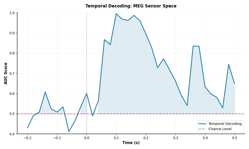
Temporal Decoding

We will emulate the temporal decoding of the original MNE tutorial. The hyperparameters chosen were experimentally found to reproduce the results of the original tutorial.

EPOCHS = 30
sliding_estimator_mlp_clf = EEGClassifier(
    BasicMLP,
    module__n_chans=n_chans,
    module__n_outputs=n_classes,
    module__n_times=1,
    criterion=nn.CrossEntropyLoss,
    optimizer=AdamW,
    optimizer__lr=0.01,
    # Note that the total dataset size is 123, but when set to 123,
    # the model actually performs significantly worse than the original MNE tutorial.
    # This is interesting because batch norm would then be equivalent
    # to the standard scaler in sklearn.
    # An interesting TODO is investigate is why?
    # Perhaps due to numerical instability?
    batch_size=8,
    max_epochs=EPOCHS,
    callbacks=[
        "accuracy",
        ("lr_scheduler", LRScheduler("CosineAnnealingLR", T_max=EPOCHS - 1)),
    ],
    device=device,
    classes=classes,
    verbose=False,  # Otherwise it would print out every training run for each time point
)

# n_jobs=1 because PyTorch models cannot be pickled and pickling is called by joblib when n_jobs > 1
time_decoding_mlp = SlidingEstimator(
    sliding_estimator_mlp_clf, n_jobs=1, scoring="roc_auc", verbose=True
)

scores = cross_val_multiscore(time_decoding_mlp, X, y_encod, cv=5, n_jobs=1)

# Mean scores across cross-validation splits
scores = np.mean(scores, axis=0)

# Plot
fig, ax = plt.subplots(figsize=(10, 6))
ax.plot(epochs.times, scores, label="Temporal Decoding", linewidth=2.5, color="#2E86AB")
ax.axhline(
    0.5, color="#A23B72", linestyle="--", linewidth=1.8, label="Chance Level", alpha=0.8
)
ax.fill_between(
    epochs.times, 0.5, scores, where=(scores >= 0.5), alpha=0.15, color="#2E86AB"
)
ax.set_xlabel("Time (s)", fontsize=11, fontweight="bold")
ax.set_ylabel("AUC Score", fontsize=11, fontweight="bold")
ax.legend(loc="lower right", frameon=True, shadow=False, fancybox=False)
ax.axvline(0.0, color="gray", linestyle="-", linewidth=1, alpha=0.5)
ax.set_title(
    "Temporal Decoding: MEG Sensor Space", fontsize=12, fontweight="bold", pad=15
)
ax.grid(True, alpha=0.3, linestyle="-", linewidth=0.5)
ax.set_ylim([0.4, 1.0])
fig.tight_layout()

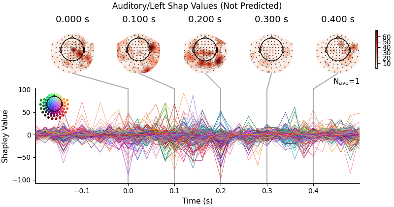
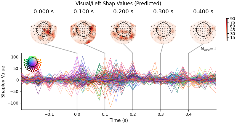
(Optional) Analyzing the spatial filters/patterns via Shapley Values

You will need to install the shap package to run this part of the tutorial. > pip install shap

In the original tutorial, the model analyzed was a LogisticRegression model, which is a linear classifier. Because our deep learning model is a non-linear classifier, we cannot use the same approach to analyze the spatial filters/patterns. However, we can still use the Shapley Values approach to analyze the spatial filters/patterns. The idea is to use the Shapley Values to estimate the importance of each feature (i.e. each channel) in the models’ decision making at each time point. We will only calculate the Shapley Values for one sample for the sake of simplicity. For this part, you will need to install the shap package (URL: https://shap.readthedocs.io/) [4].

time_decoding_mlp = time_decoding_mlp.fit(X, y_encod)

# We will use the first 100 samples as background
background = torch.from_numpy(X[:100]).to(device).to(torch.float32)
# We will use the 101st sample for demonstration
test_images = torch.from_numpy(X[100:101]).to(device).to(torch.float32)
# Note that the model predicted "visual left" for the 101st sample
print(X.shape, background.shape, test_images.shape, y_encod[100:101])
aud_shap = []
vis_shap = []

for ei, this_est in enumerate(time_decoding_mlp.estimators_):
    e = shap.DeepExplainer(this_est.module_.model, background[:, :, ei])
    shap_values = e.shap_values(test_images[:, :, ei])
    aud_shap.append(shap_values[0, :, 0])
    vis_shap.append(shap_values[0, :, 1])
aud_shap = np.asarray(aud_shap)
vis_shap = np.asarray(vis_shap)

(123, 203, 36) torch.Size([100, 203, 36]) torch.Size([1, 203, 36]) [1]

Note that we have to plot two plots because there are two outputs (auditory and visual). The higher the magnitude of the Shapley Value, the more important the feature is for making the prediction. The more positive the Shapley Value, the more the model associated that feature with the target. The more negative the Shapley Value, the less the model associated that feature with the target.

def plot_evoked(data, title):
    data = np.transpose(data)
    evoked_time_gen = mne.EvokedArray(data, epochs.info, tmin=epochs.times[0])
    joint_kwargs = dict(
        ts_args=dict(time_unit="s", units=dict(grad="Shapley Value")),
        topomap_args=dict(time_unit="s"),
    )
    evoked_time_gen.plot_joint(
        times=np.arange(0.0, 0.500, 0.100), title=title, **joint_kwargs
    )

Plot the Shapley Values for the auditory/left.

plot_evoked(aud_shap, "Auditory/Left Shap Values (Not Predicted)")

Plot the Shapley Values for the visual/left.

plot_evoked(vis_shap, "Visual/Left Shap Values (Predicted)")

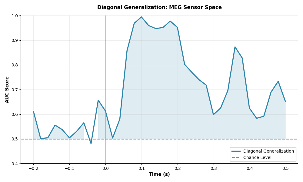
Temporal Generalization

Next, we will similarly emulate the temporal generalization of the original MNE tutorial, which is an extension of the temporal decoding approach. Instead of just predicting the target at each time point, it evaluates how well a model at a particular time point predicts the target at all other time points. Thus, instead of using a SlidingEstimator, we will use a GeneralizingEstimator. The approach is documented in [2] and [3].

generalizing_estimator_mlp_clf = EEGClassifier(
    BasicMLP,
    module__n_chans=n_chans,
    module__n_outputs=n_classes,
    module__n_times=1,
    criterion=nn.CrossEntropyLoss,
    optimizer=AdamW,
    optimizer__lr=0.01,
    batch_size=8,
    max_epochs=EPOCHS,
    callbacks=[
        "accuracy",
        ("lr_scheduler", LRScheduler("CosineAnnealingLR", T_max=EPOCHS - 1)),
    ],
    device=device,
    classes=classes,
    verbose=False,  # Otherwise it would print out every training run for each time point
)

generalizing_decoding_mlp = GeneralizingEstimator(
    generalizing_estimator_mlp_clf, n_jobs=1, scoring="roc_auc", verbose=True
)

gen_scores = cross_val_multiscore(generalizing_decoding_mlp, X, y_encod, cv=3, n_jobs=1)

The diagonal of the generalization matrix should look like the temporal decoding scores.

# Mean scores across cross-validation splits
gen_scores = np.mean(gen_scores, axis=0)

# Plot the diagonal (it's exactly the same as the time-by-time decoding above)
fig, ax = plt.subplots(figsize=(10, 6))
ax.plot(
    epochs.times,
    np.diag(gen_scores),
    label="Diagonal Generalization",
    linewidth=2.5,
    color="#2E86AB",
)
ax.axhline(
    0.5, color="#A23B72", linestyle="--", linewidth=1.8, label="Chance Level", alpha=0.8
)
ax.fill_between(
    epochs.times,
    0.5,
    np.diag(gen_scores),
    where=(np.diag(gen_scores) >= 0.5),
    alpha=0.15,
    color="#2E86AB",
)
ax.set_xlabel("Time (s)", fontsize=11, fontweight="bold")
ax.set_ylabel("AUC Score", fontsize=11, fontweight="bold")
ax.legend(loc="lower right", frameon=True, shadow=False, fancybox=False)
ax.axvline(0.0, color="gray", linestyle="-", linewidth=1, alpha=0.5)
ax.set_title(
    "Diagonal Generalization: MEG Sensor Space", fontsize=12, fontweight="bold", pad=15
)
ax.grid(True, alpha=0.3, linestyle="-", linewidth=0.5)
ax.set_ylim([0.4, 1.0])
fig.tight_layout()

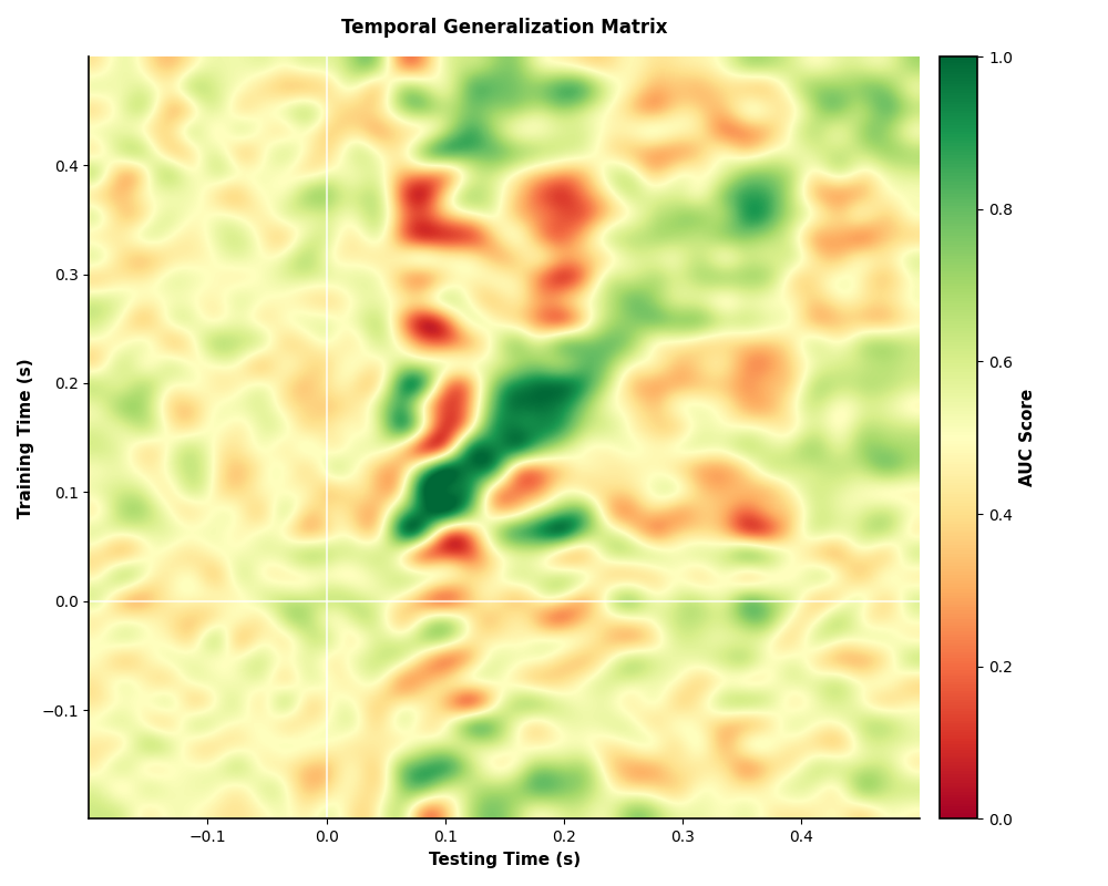
Then we plot the full generalization matrix.

fig, ax = plt.subplots(1, 1, figsize=(10, 8))
im = ax.imshow(
    gen_scores,
    interpolation="lanczos",
    origin="lower",
    cmap="RdYlGn",
    extent=epochs.times[[0, -1, 0, -1]],
    vmin=0.0,
    vmax=1.0,
    aspect="auto",
)
ax.set_xlabel("Testing Time (s)", fontsize=11, fontweight="bold")
ax.set_ylabel("Training Time (s)", fontsize=11, fontweight="bold")
ax.set_title("Temporal Generalization Matrix", fontsize=12, fontweight="bold", pad=15)
ax.axvline(0, color="white", linewidth=1.5, linestyle="-", alpha=0.7)
ax.axhline(0, color="white", linewidth=1.5, linestyle="-", alpha=0.7)
cbar = plt.colorbar(im, ax=ax, pad=0.02)
cbar.set_label("AUC Score", fontsize=11, fontweight="bold")
cbar.ax.tick_params(labelsize=10)
fig.tight_layout()

(Optional) The importance of normalization

The following is an addendum to the original MNE tutorial analalyzing how crucial normalizing is for temporal decoding/generalization. The original MNE tutorial used a StandardScaler to normalize the input data beforehand for each channel, i.e. the mean and standard deviation of each channel was computed across the entire dataset and then used to normalize each channel. You could do the same thing with an EEGClassifier by using the StandardScaler in a sklearn pipeline:

# We aren't actually going to run this
clf = make_pipeline(StandardScaler(), sliding_estimator_mlp_clf)

However, since this is a deep learning library, we wanted to use something that aligns with current deep learning practices, which is why we use a nn.BatchNorm1d layer to normalize the input channels. Let’s use another model from Braindecode, EEGSimpleConv,

class DimWrapper(nn.Module):
    """Wrapper that converts 2D input (batch, n_chans) to 3D (batch, n_chans, 1)

    Helper module because the EEGSimpleConv model expects
    input to be in the shape of (batch, n_chans, time), but since
    we are only concerned with one time point, the data passed in is
    in the shape of (batch, n_chans). This wrapper reshapes the input
    to the shape of (batch, n_chans, 1) so that the model can be
    trained on the data.
    """

    def __init__(self, model):
        super().__init__()
        self.model = model

    def forward(self, x):
        """Modify the input to be in the shape of (batch, n_chans, 1)

        X form: (batch, n_chans)
        Reshape to (batch, n_chans, 1)
        """
        if x.dim() == 2:
            x = torch.unsqueeze(x, dim=-1)
        return self.model(x)


class WrappedEEGSimpleConvNoNorm(nn.Module):
    """Wrapper that applies DimWrapper to EEGSimpleConv
    and has no batch norm module.
    """

    def __init__(
        self, n_chans, n_outputs, n_times, sfreq, feature_maps, kernel_size, n_convs
    ):
        super().__init__()
        self.eeg_simple_conv = EEGSimpleConv(
            n_chans=n_chans,
            n_outputs=n_outputs,
            n_times=n_times,
            sfreq=sfreq,
            feature_maps=feature_maps,
            kernel_size=kernel_size,
            n_convs=n_convs,
        )
        self.dim_wrapper = DimWrapper(self.eeg_simple_conv)

    def forward(self, x):
        return self.dim_wrapper(x)


class WrappedEEGSimpleConvNorm(nn.Module):
    """Wrapper that applies DimWrapper to EEGSimpleConv
    and has batch norm module.
    """

    def __init__(
        self, n_chans, n_outputs, n_times, sfreq, feature_maps, kernel_size, n_convs
    ):
        super().__init__()
        self.eeg_simple_conv = EEGSimpleConv(
            n_chans=n_chans,
            n_outputs=n_outputs,
            n_times=n_times,
            sfreq=sfreq,
            feature_maps=feature_maps,
            kernel_size=kernel_size,
            n_convs=n_convs,
        )
        self.dim_wrapper = DimWrapper(self.eeg_simple_conv)
        self.norm = nn.BatchNorm1d(n_chans, affine=False, eps=0.0)

    def forward(self, x):
        x_norm = self.norm(x)
        return self.dim_wrapper(x_norm)

Note that we have to wrap the model to include a DimWrapper and a BatchNorm1d layer. We create two different wrappers, one that applies the BatchNorm1d layer and one that does not. Now let’s perform temporal decoding with both similar to the previous example and compare the results.

Without normalization

sliding_estimator_simple_conv_no_norm_clf = EEGClassifier(
    WrappedEEGSimpleConvNoNorm,
    module__n_chans=n_chans,
    module__n_outputs=n_classes,
    module__n_times=1,
    module__sfreq=epochs.info["sfreq"],
    module__feature_maps=32,
    module__kernel_size=4,
    module__n_convs=3,
    criterion=nn.CrossEntropyLoss,
    optimizer=AdamW,
    optimizer__lr=0.01,
    batch_size=8,  # Lower batch sizes == more interesting? Why?
    max_epochs=EPOCHS,
    callbacks=[
        "accuracy",
        ("lr_scheduler", LRScheduler("CosineAnnealingLR", T_max=EPOCHS - 1)),
    ],
    device=device,
    classes=classes,
    verbose=False,  # Otherwise it would print out every training run for each time point
)

time_decoding_simple_conv_no_norm = SlidingEstimator(
    sliding_estimator_simple_conv_no_norm_clf, n_jobs=1, scoring="roc_auc", verbose=True
)

# cv = 3 for sake of speed
scores = cross_val_multiscore(
    time_decoding_simple_conv_no_norm,
    torch.from_numpy(X).to(torch.float32),
    y_encod,
    cv=3,
    n_jobs=1,
)

# Mean scores across cross-validation splits
scores = np.mean(scores, axis=0)

# Plot
fig, ax = plt.subplots(figsize=(10, 6))
ax.plot(
    epochs.times, scores, label="Without Normalization", linewidth=2.5, color="#E63946"
)
ax.axhline(
    0.5, color="#A23B72", linestyle="--", linewidth=1.8, label="Chance Level", alpha=0.8
)
ax.fill_between(
    epochs.times, 0.5, scores, where=(scores >= 0.5), alpha=0.15, color="#E63946"
)
ax.set_xlabel("Time (s)", fontsize=11, fontweight="bold")
ax.set_ylabel("AUC Score", fontsize=11, fontweight="bold")
ax.legend(loc="lower right", frameon=True, shadow=False, fancybox=False)
ax.axvline(0.0, color="gray", linestyle="-", linewidth=1, alpha=0.5)
ax.set_title(
    "EEGSimpleConv Without Normalization", fontsize=12, fontweight="bold", pad=15
)
ax.grid(True, alpha=0.3, linestyle="-", linewidth=0.5)
ax.set_ylim([0.4, 1.0])
fig.tight_layout()

With normalization

sliding_estimator_simple_conv_norm_clf = EEGClassifier(
    WrappedEEGSimpleConvNorm,
    module__n_chans=n_chans,
    module__n_outputs=n_classes,
    module__n_times=1,
    module__sfreq=epochs.info["sfreq"],
    module__feature_maps=32,
    module__kernel_size=4,
    module__n_convs=3,
    criterion=nn.CrossEntropyLoss,
    optimizer=AdamW,
    optimizer__lr=0.01,
    batch_size=8,  # Lower batch sizes == more interesting? Why?
    max_epochs=EPOCHS,
    callbacks=[
        "accuracy",
        ("lr_scheduler", LRScheduler("CosineAnnealingLR", T_max=EPOCHS - 1)),
    ],
    device=device,
    classes=classes,
    verbose=False,  # Otherwise it would print out every training run for each time point
)

time_decoding_simple_conv_norm = SlidingEstimator(
    sliding_estimator_simple_conv_norm_clf, n_jobs=1, scoring="roc_auc", verbose=True
)

# cv = 3 for sake of speed
scores = cross_val_multiscore(
    time_decoding_simple_conv_norm,
    torch.from_numpy(X).to(torch.float32),
    y_encod,
    cv=3,
    n_jobs=1,
)

# Mean scores across cross-validation splits
scores = np.mean(scores, axis=0)

# Plot
fig, ax = plt.subplots(figsize=(10, 6))
ax.plot(
    epochs.times, scores, label="With Normalization", linewidth=2.5, color="#06A77D"
)
ax.axhline(
    0.5, color="#A23B72", linestyle="--", linewidth=1.8, label="Chance Level", alpha=0.8
)
ax.fill_between(
    epochs.times, 0.5, scores, where=(scores >= 0.5), alpha=0.15, color="#06A77D"
)
ax.set_xlabel("Time (s)", fontsize=11, fontweight="bold")
ax.set_ylabel("AUC Score", fontsize=11, fontweight="bold")
ax.legend(loc="lower right", frameon=True, shadow=False, fancybox=False)
ax.axvline(0.0, color="gray", linestyle="-", linewidth=1, alpha=0.5)
ax.set_title("EEGSimpleConv With Normalization", fontsize=12, fontweight="bold", pad=15)
ax.grid(True, alpha=0.3, linestyle="-", linewidth=0.5)
ax.set_ylim([0.4, 1.0])
fig.tight_layout()

Although performing slightly worse than the previous examples, the model with normalization still resembles the original MNE tutorial. On the other hand, the model without normalization cannot effectively temporally decode at all, essentially having approximately 0.5 AUC at all time points. This suggests that normalizing the data before feeding it into the model is crucial for temporal decoding.

References

[1] (1,2)

Jean-Rémi King, Laura Gwilliams, Chris Holdgraf, Jona Sassenhagen, Alexandre Barachant, Denis Engemann, Eric Larson, and Alexandre Gramfort. “Encoding and decoding neuronal dynamics: methodological framework to uncover the algorithms of cognition.” hal-01848442, 2018. URL: https://hal.archives-ouvertes.fr/hal-01848442.

[2] (1,2)

Jean-Rémi King, Alexandre Gramfort, Aaron Schurger, Lionel Naccache, and Stanislas Dehaene. Two distinct dynamic modes subtend the detection of unexpected sounds. PLoS ONE, 9(1):e85791, 2014. URL: doi:10.1371/journal.pone.0085791.

[3] (1,2)

Jean-Rémi King and Stanislas Dehaene. Characterizing the dynamics of mental representations: the temporal generalization method. Trends in Cognitive Sciences, 18(4):203–210, 2014, URL: doi:10.1016/j.tics.2014.01.002.

[4]

Lundberg, Scott M., and Su-In Lee. “A unified approach to interpreting model predictions.” Advances in neural information processing systems 30, 2017. URL: https://dl.acm.org/doi/10.5555/3295222.3295230

Estimated memory usage: 1022 MB