
Note
Go to the end to download the full example code.
Fine-tuning a Foundation Model (Signal-JEPA)#
Foundation models are large-scale pre-trained models that serve as a starting point for a wide range of downstream tasks, leveraging their generalization capabilities. Fine-tuning these models is necessary to adapt them to specific tasks or datasets, ensuring optimal performance in specialized applications.
In this tutorial, we demonstrate how to load a pre-trained foundation model and fine-tune it for a specific task. We use the Signal-JEPA model [1] and a MOABB motor-imagery dataset for this tutorial.
# Authors: Pierre Guetschel <pierre.guetschel@gmail.com>
#
# License: BSD (3-clause)
#
import mne
import numpy as np
import torch

from braindecode import EEGClassifier
from braindecode.datasets import MOABBDataset
from braindecode.models import SignalJEPA_PreLocal
from braindecode.preprocessing import create_windows_from_events

torch.use_deterministic_algorithms(True)
torch.manual_seed(12)
np.random.seed(12)
Loading and preparing the data#
Loading a dataset#
We start by loading a MOABB dataset, a single subject only for speed. The dataset contains motor imagery EEG recordings, which we will preprocess and use for fine-tuning.
subject_id = 3  # Just one subject for speed
dataset = MOABBDataset(dataset_name="BNCI2014_001", subject_ids=[subject_id])

# Set the standard 10-20 montage for EEG channel locations
montage = mne.channels.make_standard_montage("standard_1020")
for ds in dataset.datasets:
    ds.raw.set_montage(montage)
Preprocessing to match the pretrained model#
The pretrained SignalJEPA checkpoint expects 19 EEG channels at 128 Hz with 2-second windows. We adapt the dataset accordingly: keep only EEG channels, pick the first 19, and resample.
Define Dataset parameters#
We extract the sampling frequency and channel information after preprocessing so they match the pretrained model.
sfreq = dataset.datasets[0].raw.info["sfreq"]
chs_info = dataset.datasets[0].raw.info["chs"]

print(f"{sfreq=}, {len(chs_info)=}")
sfreq=128.0, len(chs_info)=19
Create Windows from Events#
We use the create_windows_from_events function from Braindecode to segment the dataset into windows based on events.
classes = ["feet", "left_hand", "right_hand"]
classes_mapping = {c: i for i, c in enumerate(classes)}

windows_dataset = create_windows_from_events(
    dataset,
    preload=True,  # Preload the data into memory for faster processing
    mapping=classes_mapping,
    window_size_samples=256,  # 2 s at 128 Hz — matches pretrained model
    window_stride_samples=256,
)
metadata = windows_dataset.get_metadata()
print(metadata.head(10))
   i_window_in_trial  i_start_in_trial  i_stop_in_trial  ...  subject  session run
0                  0               384              640  ...        3   0train   0
1                  1               640              896  ...        3   0train   0
2                  0              1410             1666  ...        3   0train   0
3                  1              1666             1922  ...        3   0train   0
4                  0              2392             2648  ...        3   0train   0
5                  1              2648             2904  ...        3   0train   0
6                  0              3391             3647  ...        3   0train   0
7                  1              3647             3903  ...        3   0train   0
8                  0              4419             4675  ...        3   0train   0
9                  1              4675             4931  ...        3   0train   0

[10 rows x 7 columns]
Loading a pre-trained foundation model#
Load Pre-trained Weights from the Hub#
We load the pre-trained SignalJEPA downstream model from the Hugging Face
Hub using from_pretrained. The SignalJEPA_PreLocal checkpoint
already bundles the SSL backbone together with the downstream
classification layers, so a single call is all that is needed.
For other foundation models (BENDR, BIOT, Labram, STEEGFormer, etc.) the
same one-line pattern applies — see Loading and Adapting Pretrained Foundation Models. For
example, the braindecode re-host of the STEEGFormer small checkpoint can be
loaded as STEEGFormer.from_pretrained("braindecode/STEEGFormer-small",
n_outputs=len(classes), chs_info=chs_info) – pass n_outputs to size the
classification head and chs_info to align your montage with the channel
vocabulary.
model = SignalJEPA_PreLocal.from_pretrained(
    "braindecode/signal-jepa_without-chans",
    n_chans=19,
    n_times=256,
    n_outputs=len(classes),
    strict=False,
)
print(model)
======================================================================================================================================================
Layer (type (var_name):depth-idx)                  Input Shape               Output Shape              Param #                   Kernel Shape
======================================================================================================================================================
SignalJEPA_PreLocal (SignalJEPA_PreLocal)          [1, 19, 256]              [1, 3]                    --                        --
├─Sequential (spatial_conv): 1-1                   [1, 19, 256]              [1, 4, 256]               --                        --
│    └─Rearrange (0): 2-1                          [1, 19, 256]              [1, 1, 19, 256]           --                        --
│    └─Conv2d (1): 2-2                             [1, 1, 19, 256]           [1, 4, 1, 256]            80                        [19, 1]
│    └─Rearrange (2): 2-3                          [1, 4, 1, 256]            [1, 4, 256]               --                        --
├─_ConvFeatureEncoder (feature_encoder): 1-2       [1, 4, 256]               [1, 4, 64]                --                        --
│    └─Rearrange (0): 2-4                          [1, 4, 256]               [4, 1, 256]               --                        --
│    └─Sequential (1): 2-5                         [4, 1, 256]               [4, 8, 29]                --                        --
│    │    └─Conv1d (0): 3-1                        [4, 1, 256]               [4, 8, 29]                256                       [32]
│    │    └─Dropout (1): 3-2                       [4, 8, 29]                [4, 8, 29]                --                        --
│    │    └─GroupNorm (2): 3-3                     [4, 8, 29]                [4, 8, 29]                16                        --
│    │    └─GELU (3): 3-4                          [4, 8, 29]                [4, 8, 29]                --                        --
│    └─Sequential (2): 2-6                         [4, 8, 29]                [4, 16, 14]               --                        --
│    │    └─Conv1d (0): 3-5                        [4, 8, 29]                [4, 16, 14]               256                       [2]
│    │    └─Dropout (1): 3-6                       [4, 16, 14]               [4, 16, 14]               --                        --
│    │    └─GELU (2): 3-7                          [4, 16, 14]               [4, 16, 14]               --                        --
│    └─Sequential (3): 2-7                         [4, 16, 14]               [4, 32, 7]                --                        --
│    │    └─Conv1d (0): 3-8                        [4, 16, 14]               [4, 32, 7]                1,024                     [2]
│    │    └─Dropout (1): 3-9                       [4, 32, 7]                [4, 32, 7]                --                        --
│    │    └─GELU (2): 3-10                         [4, 32, 7]                [4, 32, 7]                --                        --
│    └─Sequential (4): 2-8                         [4, 32, 7]                [4, 64, 3]                --                        --
│    │    └─Conv1d (0): 3-11                       [4, 32, 7]                [4, 64, 3]                4,096                     [2]
│    │    └─Dropout (1): 3-12                      [4, 64, 3]                [4, 64, 3]                --                        --
│    │    └─GELU (2): 3-13                         [4, 64, 3]                [4, 64, 3]                --                        --
│    └─Sequential (5): 2-9                         [4, 64, 3]                [4, 64, 1]                --                        --
│    │    └─Conv1d (0): 3-14                       [4, 64, 3]                [4, 64, 1]                8,192                     [2]
│    │    └─Dropout (1): 3-15                      [4, 64, 1]                [4, 64, 1]                --                        --
│    │    └─GELU (2): 3-16                         [4, 64, 1]                [4, 64, 1]                --                        --
│    └─Rearrange (6): 2-10                         [4, 64, 1]                [1, 4, 64]                --                        --
├─Sequential (final_layer): 1-3                    [1, 4, 64]                [1, 3]                    --                        --
│    └─Flatten (0): 2-11                           [1, 4, 64]                [1, 256]                  --                        --
│    └─Linear (1): 2-12                            [1, 256]                  [1, 3]                    771                       --
======================================================================================================================================================
Total params: 14,691
Trainable params: 14,691
Non-trainable params: 0
Total mult-adds (Units.MEGABYTES): 0.18
======================================================================================================================================================
Input size (MB): 0.02
Forward/backward pass size (MB): 0.05
Params size (MB): 0.06
Estimated Total Size (MB): 0.12
======================================================================================================================================================
Fine-tuning the Model#
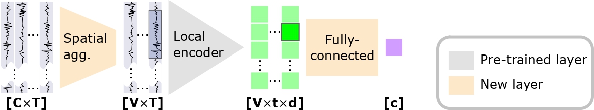
Signal-JEPA is a model trained in a self-supervised manner on a masked
prediction task. In this task, the model is configured in a many-to-many
fashion, which is not suited for a classification task. Therefore, we need to
adjust the model architecture for finetuning. This is what is done by the
SignalJEPA_PreLocal, SignalJEPA_Contextual, and
SignalJEPA_PostLocal classes. In these classes, new layers are added
specifically for classification, as described in the article [1] and in the following figure:
With this downstream architecture, two options are possible for fine-tuning:
Fine-tune only the newly added layers
Fine-tune the entire model
Freezing Pre-trained Layers#
As the second option is rather straightforward to implement, we will focus on the first option here. We will freeze all layers except the newly added ones.
# Keep the task-specific head layers (spatial_conv and final_layer)
# trainable and freeze the pretrained backbone.
new_layers = {
    name
    for name, _ in model.named_parameters()
    if name.startswith(("spatial_conv.", "final_layer."))
}

for name, param in model.named_parameters():
    if name not in new_layers:
        param.requires_grad = False

print("Trainable parameters:")
other_modules = set()
for name, param in model.named_parameters():
    if param.requires_grad:
        print(name)
    else:
        other_modules.add(name.split(".")[0])

print("\nOther modules:")
print(other_modules)
Trainable parameters:
spatial_conv.1.weight
spatial_conv.1.bias
final_layer.1.weight
final_layer.1.bias

Other modules:
{'feature_encoder'}
Fine-tuning Procedure#
Finally, we set up the fine-tuning procedure using Braindecode’s
EEGClassifier. We define the loss function, optimizer, and training
parameters. We then fit the model to the windows dataset.
We only train for a few epochs for demonstration purposes.
clf = EEGClassifier(
    model,
    criterion=torch.nn.CrossEntropyLoss,
    optimizer=torch.optim.AdamW,
    optimizer__lr=0.005,
    batch_size=16,
    callbacks=["accuracy"],
    classes=range(3),
)
_ = clf.fit(windows_dataset, y=metadata["target"], epochs=10)
  epoch    train_accuracy    train_loss    valid_acc    valid_accuracy    valid_loss     dur
-------  ----------------  ------------  -----------  ----------------  ------------  ------
      1            0.3343        1.0995       0.3295            0.3295        1.0987  0.2495
      2            0.3343        1.0994       0.3295            0.3295        1.0986  0.2190
      3            0.3329        1.0988       0.3353            0.3353        1.0986  0.2259
      4            0.3777        1.0984       0.3353            0.3353        1.0985  0.2255
      5            0.3878        1.0980       0.3237            0.3237        1.0984  0.2191
      6            0.4096        1.0974       0.3931            0.3931        1.0983  0.2181
      7            0.3893        1.0963       0.3295            0.3295        1.0980  0.2194
      8            0.4211        1.0952       0.3931            0.3931        1.0978  0.2190
      9            0.4356        1.0931       0.3179            0.3179        1.0975  0.2187
     10            0.4457        1.0917       0.3699            0.3699        1.0974  0.2197
All-in-one Implementation#
In the implementation above, we manually loaded the weights and froze the layers.
This forces us to pass an initialized model to EEGClassifier, which may
create issues if we use it in a cross-validation setting.
Instead, we can implement the same procedure in a more compact and reproducible way, by using skorch’s callback system.
Here, we import a callback to freeze layers and define a custom callback to load the pre-trained weights at the beginning of training:
from skorch.callbacks import Callback, Freezer


class WeightsLoader(Callback):
    def __init__(self, url, strict=False):
        self.url = url
        self.strict = strict

    def on_train_begin(self, net, X=None, y=None, **kwargs):
        state_dict = torch.hub.load_state_dict_from_url(url=self.url)
        net.module_.load_state_dict(state_dict, strict=self.strict)
We can now define a classifier with those callbacks, without having to pass an initialized model, and fit it as before:
clf = EEGClassifier(
    "SignalJEPA_PreLocal",
    criterion=torch.nn.CrossEntropyLoss,
    optimizer=torch.optim.AdamW,
    optimizer__lr=0.005,
    batch_size=16,
    callbacks=[
        "accuracy",
        WeightsLoader(
            url="https://huggingface.co/braindecode/signal-jepa_without-chans/resolve/main/pytorch_model.bin"
        ),
        Freezer(patterns="feature_encoder.*"),
    ],
    classes=range(3),
)
_ = clf.fit(windows_dataset, y=metadata["target"], epochs=10)
Downloading: "https://huggingface.co/braindecode/signal-jepa_without-chans/resolve/main/pytorch_model.bin" to /home/runner/.cache/torch/hub/checkpoints/pytorch_model.bin

  0%|          | 0.00/13.2M [00:00<?, ?B/s]
  1%|          | 128k/13.2M [00:00<00:14, 979kB/s]
  5%|▍         | 640k/13.2M [00:00<00:04, 3.05MB/s]
 14%|█▍        | 1.88M/13.2M [00:00<00:01, 7.18MB/s]
 39%|███▊      | 5.12M/13.2M [00:00<00:00, 17.1MB/s]
 80%|████████  | 10.6M/13.2M [00:00<00:00, 31.2MB/s]
100%|██████████| 13.2M/13.2M [00:00<00:00, 20.7MB/s]
  epoch    train_accuracy    train_loss    valid_acc    valid_accuracy    valid_loss     dur
-------  ----------------  ------------  -----------  ----------------  ------------  ------
      1            0.3329        1.0999       0.3353            0.3353        1.0986  0.2308
      2            0.3994        1.0990       0.3526            0.3526        1.0986  0.2213
      3            0.3372        1.0987       0.3295            0.3295        1.0986  0.2195
      4            0.4023        1.0983       0.3642            0.3642        1.0985  0.2195
      5            0.4081        1.0978       0.3815            0.3815        1.0983  0.2198
      6            0.4530        1.0967       0.3468            0.3468        1.0982  0.2192
      7            0.4399        1.0955       0.3699            0.3699        1.0980  0.2211
      8            0.4023        1.0941       0.3295            0.3295        1.0979  0.2183
      9            0.4443        1.0927       0.3584            0.3584        1.0976  0.2195
     10            0.4559        1.0911       0.3642            0.3642        1.0974  0.2193
Conclusion and Next Steps#
In this tutorial, we demonstrated how to fine-tune a pre-trained foundation model, Signal-JEPA, for a motor imagery classification task. We now have a basic implementation that can automatically load pre-trained weights and freeze specific layers.
This setup can easily be extended to explore different fine-tuning techniques, base foundation models, and downstream tasks.
References#
Total running time of the script: (0 minutes 18.575 seconds)
Estimated memory usage: 573 MB
Run this example